Authors: Rail Sabirov, Maksim Ilin, Ivan Ilyichev — Innopolis University
Recommender systems have become an integral part of our digital lives, powering content discovery on platforms ranging from streaming services to e-commerce websites. Traditional collaborative filtering methods, while effective, often struggle with cold-start problems and fail to leverage the rich relational structure inherent in recommendation data. This is where graph machine learning offers a promising alternative.
If you are familiar with machine learning but new to graph neural networks, think of them as an extension of convolutional neural networks (CNNs) that operate on graph-structured data instead of regular grids. Just as CNNs learn features by aggregating information from neighboring pixels, graph neural networks learn node representations by aggregating information from neighboring nodes in a graph. This makes them particularly well-suited for recommendation tasks, where we can naturally model users and items as nodes, and their interactions as edges.
In this work, we present a comprehensive study of graph-based approaches for movie recommendation. We analyze users' preferences and recommend movies that users might like by leveraging two different graph representations of the problem. Our system uses shrinked version of The Movies Dataset, containing information about 45.000 movies from the Full MovieLens Dataset, including genres, production companies, countries, release dates, cast, crew, and ratings from 270.000 users. For computational efficiency and effective demonstration of our approaches, we use a subset consisting of 700 users, 100.000 ratings, and 9.000 movies.
The prediction task we address is link prediction — specifically, predicting which user-movie links are likely to be favorable. We evaluate our approaches using standard classification metrics, such as accuracy, F1, ROC-AUC, etc. considering a movie as relevant if the user rated it 4 or 5 stars.
We compare three distinct approaches: (1) a content-based method with Correct-and-Smooth refinement (CS), (2) a per-user rating (label) propagation method (PRC), and (3) Graph Neural Networks (GCN and GraphSAGE). Our experiments are conducted on three different graph constructions: a cosine similarity-based graph, a UMAP-style fuzzy similarity graph, and a heterogeneous graph. Through this comprehensive evaluation, we provide insights into the relative strengths and weaknesses of each approach, offering practical guidance for practitioners working on graph-based recommendation systems.

Image credit: https://mbernste.github.io/posts/gcn/
Graph Convolutional Networks, introduced by Kipf and Welling [2], extend the concept of convolutional operations to graph-structured data. GCNs operate by learning node representations through a message-passing mechanism where each node aggregates information from its neighbors.
The core operation in a GCN layer can be expressed as:
where
where
GCNs are particularly effective for recommendation tasks because they can leverage both node features and graph structure simultaneously. In our movie recommendation context, GCNs allow movies to learn representations that incorporate information from similar movies, enabling the model to make recommendations based on content similarity and collaborative patterns.
GraphSAGE (Graph Sample and Aggregate), introduced by Hamiltom et al., is an inductive framework that learns node embeddings by sampling and aggregating feature information from a node's local neighborhood. Unlike GCN, which requires the full graph during training, GraphSAGE can generate embeddings for new nodes that were not seen during training, making it more flexible for dynamic graphs, which is more appropriate for real world recommender systems embedded into streaming services, for example.
The GraphSAGE update rule for a node
where
The key innovation of GraphSAGE is its ability to sample a fixed-size neighborhood for each node, making it computationally efficient and scalable to large graphs. This sampling strategy also provides robustness to variations in node degrees, which is particularly important in recommendation systems where some movies may have many more ratings than others.
We construct a weighted movie similarity graph using a homogeneous item-item paradigm where movies are nodes and edges represent similarity relationships. Our pipeline transforms raw movie metadata into feature vectors, builds a k-nearest neighbor (kNN) graph, and applies two different edge-weighting schemes: simple cosine-derived weights and UMAP-style fuzzy weights with symmetrization.
For the similarity graphs we use three data files:
data/movies_metadata.csv: core movie information includingid,title,adult,genres,overview,popularity,vote_average, andvote_countdata/keywords.csv: movie-level keywordsdata/links.csv: mapping betweenmovieId(MovieLens) andtmdbId(TMDB id) for identifier alignment
For the heterogeneous graph we use:
data/movies_metadata.csv: core movie information includingid,title,adult,genres,overview,popularity,vote_average, andvote_countdata/links.csv: mapping betweenmovieId(MovieLens) andtmdbId(TMDB id) for identifier alignmentdata/credits.csv: information about the film cast and crewdata/ratings.csv:: user rating
The full preprocessing pipeline for the HG is available on Google Colab: HGDataPreparation
We parse JSON-like columns, handle missing values, and enforce consistent data types. Rows missing essential fields like id or title are dropped.
# genres: convert JSON-like string to list of names
movies['genres'] = (
    movies['genres']
    .fillna('[]')
    .apply(eval)
    .apply(lambda x: [y['name'] for y in x] if isinstance(x, list) else [])
)

# keywords: join as list of names
keywords_df['keywords'] = keywords_df['keywords'].fillna('[]').apply(eval)
movies = movies.merge(keywords_df[['id', 'keywords']], on='id', how='left')
movies['keywords'] = movies['keywords'].apply(lambda x: [y['name'] for y in x] if isinstance(x, list) else [])

# drop rows missing id/title
movies.dropna(subset=['id', 'title'], inplace=True)We build a mixed representation combining text, categorical multi-labels, and numeric signals:
- Text features: Movie overviews encoded via TF-IDF (max 5,000 features)
- Categorical features: One-hot encodings for
genresandkeywordsusingMultiLabelBinarizer - Binary features:
adultflag mapped to {0, 1} - Numeric features:
popularity,vote_average, andlog1p(vote_count), all standardized
This representation captures semantic content (TF-IDF), content taxonomy (genres, keywords), and popularity/quality signals.
from sklearn.feature_extraction.text import TfidfVectorizer
from sklearn.preprocessing import MultiLabelBinarizer, StandardScaler
from scipy.sparse import hstack

# 1) Overview TF-IDF
tfidf = TfidfVectorizer(max_features=5000, stop_words='english')
movies['overview'] = movies['overview'].fillna('')
tfidf_matrix = tfidf.fit_transform(movies['overview'])

# 2) Genres / 3) Keywords
mlb_genres = MultiLabelBinarizer()
genres_m = mlb_genres.fit_transform(movies['genres'])
mlb_keywords = MultiLabelBinarizer()
keywords_m = mlb_keywords.fit_transform(movies['keywords'])

# 4) Adult flag
adult_mask = movies['adult'].fillna('False').map({'True': 1, 'False': 0}).values.reshape(-1, 1)

# 5) Numeric
numeric_features = movies[['popularity', 'vote_average', 'vote_count']].fillna(0)
numeric_features['popularity'] = pd.to_numeric(numeric_features['popularity'], errors='coerce').fillna(0)
numeric_features['vote_count'] = np.log1p(numeric_features['vote_count'])
scaler = StandardScaler()
numeric_m = scaler.fit_transform(numeric_features)

# Combined sparse feature matrix
X = hstack([tfidf_matrix, genres_m, keywords_m, adult_mask, numeric_m])We construct mapping dictionaries to connect the relationships between nodes:
movie_id_to_idx = {movie_id: idx for idx, movie_id in enumerate(df_connections_movie_features['movie_id'].unique())}
user_id_to_idx = {user_id: idx for idx, user_id in enumerate(df_connections_user_stats['user_id'].unique())}
director_id_to_idx = {director_id: idx for idx, director_id in
                      enumerate(df_connections_directors['director_id'].unique())}
actor_id_to_idx = {actor_id: idx for idx, actor_id in enumerate(df_connections_actors['actor_id'].unique())}
genre_id_to_idx = {genre_id: idx for idx, genre_id in enumerate(df_connections_genres['genre_id'].unique())}
Then, in order to speed up the computations, we are considering top-5000 users according to the amount of rated films. Such approach allows for obtaining more data to learn for each user. Using the function we create a subgraph of the original:
def build_subgraph_for_users(
        user_ids,
        df_user_movie,
        df_movie_features,
        df_user_stats,
        df_movie_genre,
        df_movie_actor,
        df_movie_director,
        df_actors,
        df_directors,
        df_genres,
        num_negatives=200
):
    selected_users = set(user_ids)
    df_user_stats_sub = df_user_stats[df_user_stats['user_id'].isin(selected_users)].copy()

    df_user_movie_sub = df_user_movie[df_user_movie['user_id'].isin(selected_users)].copy()
    selected_movie_ids = set(df_user_movie_sub['movie_id'].unique())

    df_movie_features_sub = df_movie_features[df_movie_features['movie_id'].isin(selected_movie_ids)].copy()
    df_movie_genre_sub = df_movie_genre[df_movie_genre['movie_id'].isin(selected_movie_ids)].copy()
    df_movie_actor_sub = df_movie_actor[df_movie_actor['movie_id'].isin(selected_movie_ids)].copy()
    df_movie_director_sub = df_movie_director[df_movie_director['movie_id'].isin(selected_movie_ids)].copy()

    selected_genre_ids = set(df_movie_genre_sub['genre_id'].unique())
    selected_actor_ids = set(df_movie_actor_sub['actor_id'].unique())
    selected_director_ids = set(df_movie_director_sub['director_id'].unique())

    df_genres_sub = df_genres[df_genres['genre_id'].isin(selected_genre_ids)].copy()
    df_actors_sub = df_actors[df_actors['actor_id'].isin(selected_actor_ids)].copy()
    df_directors_sub = df_directors[df_directors['director_id'].isin(selected_director_ids)].copy()

    print(f'\nSizes of filtered data:')
    print(f'Users: {df_user_stats_sub.shape[0]}')
    print(f'Movies: {df_movie_features_sub.shape[0]}')
    print(f'User-movie links: {df_user_movie_sub.shape[0]}')
    print(f'Actors: {df_actors_sub.shape[0]}')
    print(f'Directors: {df_directors_sub.shape[0]}')
    print(f'Genres: {df_genres_sub.shape[0]}')

    scaler = StandardScaler()

    movie_num_cols = ['vote_average', 'vote_count', 'popularity']
    if len(df_movie_features_sub) > 0:
        df_movie_features_sub[movie_num_cols] = scaler.fit_transform(
            df_movie_features_sub[movie_num_cols].fillna(0)
        )

    user_num_cols = ['num_ratings', 'avg_rating', 'activity_days']
    if len(df_user_stats_sub) > 0:
        df_user_stats_sub[user_num_cols] = scaler.fit_transform(
            df_user_stats_sub[user_num_cols].fillna(0)
        )

    if len(df_directors_sub) > 0:
        df_directors_sub['total_films'] = scaler.fit_transform(
            df_directors_sub[['total_films']].fillna(0)
        )

    actor_num_cols = ['total_films', 'avg_order']
    if len(df_actors_sub) > 0:
        df_actors_sub[actor_num_cols] = scaler.fit_transform(
            df_actors_sub[actor_num_cols].fillna(0)
        )

    gender_encoder = OneHotEncoder(sparse_output=False, categories=[[0, 1, 2]], handle_unknown='ignore')
    if len(df_directors_sub) > 0:
        gender_dir_encoded = gender_encoder.fit_transform(df_directors_sub[['gender']])
        gender_dir_df = pd.DataFrame(gender_dir_encoded,
                                     columns=['gender_0', 'gender_1', 'gender_2'])
        df_directors_sub = pd.concat([df_directors_sub.reset_index(drop=True),
                                      gender_dir_df], axis=1)
        df_directors_sub = df_directors_sub.drop('gender', axis=1)

    if len(df_actors_sub) > 0:
        gender_act_encoded = gender_encoder.transform(df_actors_sub[['gender']])
        gender_act_df = pd.DataFrame(gender_act_encoded,
                                     columns=['gender_0', 'gender_1', 'gender_2'])
        df_actors_sub = pd.concat([df_actors_sub.reset_index(drop=True),
                                   gender_act_df], axis=1)
        df_actors_sub = df_actors_sub.drop('gender', axis=1)

    if len(df_genres_sub) > 0:
        genre_encoder = OneHotEncoder(sparse_output=False)
        genre_encoded = genre_encoder.fit_transform(df_genres_sub[['genre_id']])
        genre_cols = [f'genre_{int(i)}' for i in genre_encoder.categories_[0]]
        genre_df = pd.DataFrame(genre_encoded, columns=genre_cols)
        df_genres_sub = pd.concat([df_genres_sub.reset_index(drop=True),
                                   genre_df], axis=1)
        df_genres_sub = df_genres_sub.drop('genre_name', axis=1)

    mappings = {}
    mappings['user'] = {user_id: idx for idx, user_id in enumerate(df_user_stats_sub['user_id'].unique())}
    mappings['movie'] = {movie_id: idx for idx, movie_id in enumerate(df_movie_features_sub['movie_id'].unique())}
    mappings['actor'] = {actor_id: idx for idx, actor_id in enumerate(df_actors_sub['actor_id'].unique())}
    mappings['director'] = {director_id: idx for idx, director_id in
                            enumerate(df_directors_sub['director_id'].unique())}
    mappings['genre'] = {genre_id: idx for idx, genre_id in enumerate(df_genres_sub['genre_id'].unique())}

    data = HeteroData()
    data['user'].num_nodes = len(mappings['user'])
    data['movie'].num_nodes = len(mappings['movie'])
    data['actor'].num_nodes = len(mappings['actor'])
    data['director'].num_nodes = len(mappings['director'])
    data['genre'].num_nodes = len(mappings['genre'])

    def add_node_features(df, node_type, id_col, mapping, data_obj):
        if len(df) == 0:
            return

        features_list = []
        feature_cols = [col for col in df.columns if col != id_col]
        sorted_ids = sorted(mapping.keys(), key=lambda x: mapping[x])
        for node_id in sorted_ids:
            row = df[df[id_col] == node_id]
            if len(row) > 0:
                features = row[feature_cols].values[0].astype(np.float32)
                features_list.append(features)
            else:
                features_list.append(np.zeros(len(feature_cols), dtype=np.float32))
        data_obj[node_type].x = torch.tensor(np.array(features_list), dtype=torch.float32)

    add_node_features(df_user_stats_sub, 'user', 'user_id', mappings['user'], data)
    add_node_features(df_movie_features_sub, 'movie', 'movie_id', mappings['movie'], data)
    add_node_features(df_actors_sub, 'actor', 'actor_id', mappings['actor'], data)
    add_node_features(df_directors_sub, 'director', 'director_id', mappings['director'], data)
    add_node_features(df_genres_sub, 'genre', 'genre_id', mappings['genre'], data)

    def add_edges(df, source_type, target_type, source_col, target_col,
                  edge_type_name, data_obj, mappings_dict, weight_col=None):
        if len(df) == 0:
            return

        edges = []
        weights = [] if weight_col is not None else None
        for _, row in df.iterrows():
            source_idx = mappings_dict[source_type].get(row[source_col])
            target_idx = mappings_dict[target_type].get(row[target_col])
            if source_idx is not None and target_idx is not None:
                edges.append([source_idx, target_idx])
                if weight_col is not None:
                    weights.append(row[weight_col])

        if edges:
            edge_tensor = torch.tensor(edges, dtype=torch.long).t().contiguous()
            data_obj[source_type, edge_type_name, target_type].edge_index = edge_tensor
            if weights is not None:
                data_obj[source_type, edge_type_name, target_type].edge_weight = torch.tensor(
                    weights, dtype=torch.float32
                )

    add_edges(df_user_movie_sub, 'user', 'movie', 'user_id', 'movie_id',
              'rates', data, mappings, weight_col='rating')
    add_edges(df_movie_genre_sub, 'movie', 'genre', 'movie_id', 'genre_id',
              'has_genre', data, mappings)
    add_edges(df_movie_director_sub, 'movie', 'director', 'movie_id', 'director_id',
              'has_director', data, mappings)
    add_edges(df_movie_actor_sub, 'movie', 'actor', 'movie_id', 'actor_id',
              'has_actor', data, mappings, weight_col='weight')

    edge_types_to_reverse = [
        ('movie', 'has_genre', 'genre'),
        ('movie', 'has_director', 'director'),
        ('movie', 'has_actor', 'actor'),
        ('user', 'rates', 'movie')
    ]

    for src, rel, dst in edge_types_to_reverse:
        if hasattr(data[src, rel, dst], 'edge_index'):
            reverse_edges = data[src, rel, dst].edge_index[[1, 0]]
            rev_rel = f'rev_{rel}'
            data[dst, rev_rel, src].edge_index = reverse_edges
            if hasattr(data[src, rel, dst], 'edge_weight'):
                data[dst, rev_rel, src].edge_weight = data[src, rel, dst].edge_weight

    print(f'\nConstructed graph with the following structure:')
    print(f'Nodes: {data.node_types}')
    print(f'Edges: {data.edge_types}')
    print(f'\nChecking node features:')

    for node_type in data.node_types:
        if hasattr(data[node_type], 'x'):
            print(f'  {node_type}: {data[node_type].x.shape}')

    print(f'\nChecking edges:')
    for edge_type in data.edge_types:
        if hasattr(data[edge_type], 'edge_index'):
            print(f'  {edge_type}: {data[edge_type].edge_index.shape[1]} edges')
return data, mappings, df_user_movie_subWe construct a kNN graph using cosine distance on the combined sparse features. For each movie, we connect to its top
from sklearn.neighbors import NearestNeighbors

k = 20
nn = NearestNeighbors(n_neighbors=k, metric='cosine').fit(X)
distances, neighbors = nn.kneighbors(X)

edge_list = []
for i in range(len(movies)):
    movie_i_id = movies.iloc[i]['id']
    for idx, j in enumerate(neighbors[i]):
        if i == j:
            continue
        movie_j_id = movies.iloc[j]['id']
        dist = distances[i][idx]
        weight = 1 - dist  # cosine similarity
        edge_list.append((movie_i_id, movie_j_id, weight))

edges_df = pd.DataFrame(edge_list, columns=['source', 'target', 'weight'])
edges_df.to_csv('processed_data/movie_similarity_graph.csv', index=False)
The cosine metric works well with high-dimensional sparse TF-IDF features. The resulting graph is directed by construction but can be symmetrized if needed.
The second approach applies UMAP-style fuzzy weighting to create more informative edge weights that adapt to local density. This method prevents dense regions from becoming over-connected while ensuring sparse regions maintain adequate connectivity.
The algorithm proceeds in four steps:
-
Local connectivity (
$\rho_i$ ): For each node$i$ , set$\rho_i$ to the smallest non-zero neighbor distance. This guarantees at least one strong local edge. -
Per-node scale (
$\sigma_i$ ): Find$\sigma_i$ via binary search such that the total affinity "mass" around$i$ equals$\log_2(k)$ :
The
-
Directional fuzzy weights: Compute
$w_{ij} = \exp\left(-\frac{d_{ij} - \rho_i}{\sigma_i}\right)$ -
Symmetrization: Apply probabilistic union
$w_{ij} = 1 - (1 - w_{ij}) \cdot (1 - w_{ji})$ so an undirected edge is strong if either direction is strong.
n = X.shape[0]
rhos = np.zeros(n)
sigmas = np.zeros(n)

for i in range(n):
    d = distances[i]
    d_nonzero = d[d > 0]
    rhos[i] = np.min(d_nonzero) if len(d_nonzero) else 0
    target = np.log2(k)
    low, high = 1e-3, 10
    for _ in range(50):
        mid = (low + high) / 2
        sum_w = np.sum(np.exp(-(d - rhos[i]) / mid))
        if abs(sum_w - target) < 1e-3:
            break
        if sum_w > target:
            high = mid
        else:
            low = mid
    sigmas[i] = mid

# directional weights
rows = []
for i in range(n):
    movie_i = movies.iloc[i]['id']
    for idx, j in enumerate(neighbors[i]):
        if i == j:
            continue
        movie_j = movies.iloc[j]['id']
        d = distances[i][idx]
        w = np.exp(-(d - rhos[i]) / sigmas[i])
        rows.append((movie_i, movie_j, w))

df = pd.DataFrame(rows, columns=['source', 'target', 'weight'])

# symmetric union
df_rev = df.rename(columns={'source':'target', 'target':'source', 'weight':'w_rev'})
dfm = df.merge(df_rev, on=['source','target'], how='outer').fillna(0)
dfm['weight'] = 1 - (1 - dfm['weight']) * (1 - dfm['w_rev'])

edges_final = dfm[['source', 'target', 'weight']]
edges_final = edges_final[edges_final['source'] != edges_final['target']]

edges_final.to_csv('processed_data/umap_movie_graph.csv', index=False)
This approach yields smoother, locally balanced neighborhoods that better reflect the underlying data topology.
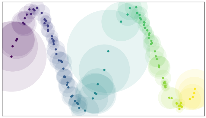
Image credit: UMAP Documentation
For computational efficiency of the similarity graphs, we drop zero-weight edges and save compact versions for downstream training:
edges_final = edges_final[edges_final['weight'] > 0]
edges_final.to_csv('processed_data/umap_movie_graph_truncated.csv', index=False)
On the other hand, for the heterogeneous graph we sample the users from the initial distribution such that their amount of rated movies lie between 25th and 75th percentiles. Then, as was mentioned earlier, the sample is taken over this set. Thus, we obtain the users with "common" amount of rated films that helps us to avoid such cases as cold start (it can be considered as a future implication).
Downstream models can consume either processed_data/movie_similarity_graph.csv (cosine-based) or processed_data/umap_movie_graph_truncated.csv (UMAP-style affinities).
Key parameters to consider for the similarity graphs:
-
$k$ (neighbors per node): 10–50 is typical; higher$k$ increases graph density and computation cost -
max_featuresin TF-IDF: balances vocabulary richness versus memory usage -
Numeric scaling: always standardize; use
log1pon heavy-tailed counts like vote counts -
UMAP target:
$\log_2(k)$ is standard from UMAP literature but can be tuned
Reproducibility: scikit-learn's NearestNeighbors is deterministic given inputs; randomness primarily arises from sampling and floating-point non-determinism across different BLAS backends.
Key parameters to consider for the heterogeneous graph:
- num_negatives: the parameter should be chosen according to the amount of movies. The higher value leads to more hits and higher computational complexity.
- max_users: the maximal amount of the validation set. The parameter also affects the metrics values. The higher value leads to more hits and higher computational complexity.
Our baseline approach trains a global item-user embedding model that learns shared content representations while personalizing to individual users. This method combines the efficiency of content-based filtering with graph-aware refinement.
Per-User Binary Labels
We create binary labels by thresholding each user's ratings at their personal mean, ensuring fair comparison across users with different rating scales:
ratings = ratings.groupby('userId', group_keys=False).apply(
    lambda df: df.assign(label=(df['rating'] >= df['rating'].mean()).astype(int))
)
This personal mean thresholding adapts automatically to users who rate high or low globally, avoiding bias toward any particular rating style.
Model Architecture
The model consists of a shared item encoder and per-user embeddings:
class ItemUserModel(nn.Module):
    def __init__(self, in_dim, emb_dim, n_users, hidden_dim=256, dropout=0.2):
        self.item_net = nn.Sequential(
            nn.Linear(in_dim, hidden_dim),
            nn.ReLU(),
            nn.Dropout(dropout),
            nn.Linear(hidden_dim, emb_dim)
        )
        self.user_emb = nn.Embedding(n_users, emb_dim)
        self.user_bias = nn.Embedding(n_users, 1)

    def forward(self, Xb, user_idx):
        h = self.item_net(Xb)         # item embedding
        u = self.user_emb(user_idx)   # user embedding
        b = self.user_bias(user_idx).squeeze(-1)
        logit = (h * u).sum(dim=1) + b
        return logit, h
The shared item encoder (item_net) maps sparse movie features to dense embeddings, learning universal content representations from all users. Per-user embeddings (user_emb) and biases (user_bias) capture individual preferences. The model predicts compatibility using a dot product:
Graph Normalization
Before applying graph-based refinement, we normalize the adjacency matrix to prevent degree bias:
A = coo_matrix((weights, (src_idx, dst_idx)), shape=(X.shape[0], X.shape[0])).tocsr()
if CFG['symmetrize_graph']:
    A = (A + A.T) * 0.5
row_sums = np.asarray(A.sum(axis=1)).reshape(-1)
row_sums[row_sums == 0] = 1.0
D_inv = csr_matrix((1/row_sums, (np.arange(len(row_sums)), np.arange(len(row_sums)))), shape=A.shape)
A_norm = D_inv.dot(A)
Symmetrization ensures mutual similarity, while row-normalization ensures each node's influence is normalized during smoothing.
Correct-and-Smooth Refinement
After obtaining base predictions from the trained model, we apply a two-stage refinement that leverages the graph structure:
-
Correction: Adjust predictions on labeled training items toward their true labels:
y_corr = y_soft.copy()
y_corr[train_idx] += alpha * (y_train - y_soft[train_idx])
where
$\alpha = 0.8$ controls the strength of correction. This anchors predictions at known labels without retraining the model. -
Smoothing: Diffuse corrected scores across the graph using iterative neighborhood averaging:
y_sm = y_corr.copy()
for _ in range(T):
    y_neigh = A_norm.dot(y_sm)
    y_sm = (1-beta)*y_sm + beta*y_neigh
where
$\hat{A}$ is the row-normalized adjacency matrix,$\beta = 0.5$ balances self-information with neighborhood influence, and$T=1$ iteration reduces oversmoothing risk while adding collaborative signal.
This refinement process is computationally cheap and improves personalization by propagating user preferences through the movie similarity graph.
This simple yet effective approach performs label propagation on the movie similarity graph without requiring any neural network training. For each user, we propagate their preferences from rated movies to unrated ones through the graph structure.
Problem Framing
We predict whether a user will like a movie (binary label) using the content-derived movie similarity graph. Each user has a small set of labeled nodes (movies they rated), and we need to infer beliefs for unseen movies. This approach is cold-start resilient since it relies on content/graph features rather than collaborative filtering.
Data Preparation
We load the movie similarity graph and convert it to an adjacency dictionary for efficient neighbor lookups:
merged = pd.read_csv('processed_data/ratings_with_tmdb.csv')
movie_sim_graph = pd.read_csv('processed_data/umap_movie_graph_truncated.csv')
adj = movie_sim_graph.groupby('source').apply(
    lambda df: list(zip(df['target'], df['weight']))
).to_dict()
Per-User Binarization
Similar to the CSR approach, we create binary labels by thresholding each user's ratings at their personal mean:
for user, user_df in merged.groupby('userId'):
    mean_r = user_df['rating'].mean()
    user_df['label'] = (user_df['rating'] >= mean_r).astype(int)
    if user_df.shape[0] < 10:
        continue
This normalizes personal rating scales and avoids bias toward users who rate globally high or low. We require at least 10 interactions per user for stability.
Train/Test Split
For each user, we sample 80% of interactions for training and keep 20% for testing:
train = user_df.sample(frac=0.8, random_state=42)
test = user_df.drop(train.index)
if len(test) < 5:
    continue
We ensure the test set has at least 5 items to compute stable metrics.
Initialization and Propagation
We initialize beliefs as follows:
- Training items: belief = true label (0 or 1)
- Test items: belief = 0.5 (uninformative prior)
The 0.5 prior encodes uncertainty rather than assuming negative or positive, preventing bias before diffusion begins.
Propagation iteratively updates test node beliefs by weighted averaging of neighbor beliefs:
iterations = 50
beliefs = {}
for _, r in train.iterrows():
    beliefs[r['tmdbId']] = float(r['label'])

test_movies = test['tmdbId'].tolist()
for m in test_movies:
    beliefs[m] = 0.5

for _ in range(iterations):
    new_beliefs = beliefs.copy()
    for m in test_movies:
        neighbors = adj.get(m, [])
        if not neighbors:
            continue
        num = 0
        den = 0
        for nb, w in neighbors:
            if nb in beliefs:
                num += w * beliefs[nb]
                den += w
        if den > 0:
            new_beliefs[m] = num / den

    if max(abs(new_beliefs[m] - beliefs[m]) for m in test_movies) < 1e-4:
        break
    beliefs = new_beliefs
The update rule can be expressed mathematically as:
where:
-
$b_i^{(t+1)}$ is the updated belief for node$i$ at iteration$t+1$ -
$\mathcal{N}(i)$ represents the set of neighbors of node$i$ in the graph -
$w_{ij}$ is the edge weight between nodes$i$ and$j$ (movie similarity) -
$b_j^{(t)}$ is the current belief of neighbor$j$ at iteration$t$ - The numerator computes the weighted sum of neighbor beliefs
- The denominator normalizes by the sum of edge weights, ensuring the update is a weighted average
This neighbor-weighted averaging approximates harmonic functions on graphs, where unlabeled nodes converge to a smooth labeling consistent with labeled boundary conditions. The process converges when the maximum change in beliefs falls below
Prediction and Evaluation
After convergence, we compute predictions and metrics:
y_true = test['label'].values
y_score = np.array([beliefs[m] for m in test_movies])
y_pred = (y_score >= 0.5).astype(int)

results.append({
    'userId': user,
    'accuracy': accuracy_score(y_true, y_pred),
    'f1': f1_score(y_true, y_pred, zero_division=0),
    'roc_auc': roc_auc_score(y_true, y_score) if len(np.unique(y_true))>1 else np.nan,
    'precision': precision_score(y_true, y_pred),
    'recall': recall_score(y_true, y_pred),
    'train_size': len(train),
    'test_size': len(test),
})
This method leverages the graph structure to propagate user preferences from rated movies to unrated ones, providing a strong baseline that requires no neural net work training. It's particularly interpretable since beliefs diffuse through similar movies with weights reflecting content similarity.
The details on technique implementation are provided as follows on Google Colab: Probabilistic Relational Classifier Notebook
We implement two GNN architectures (GCN and GraphSAGE) using PyTorch Geometric to learn node representations that combine content features with graph structure. Unlike the previous approaches, GNNs learn end-to-end functions that propagate label information across similar movies through learned message-passing operations.
Why GNNs for Recommendation
GNNs enable label information to propagate across similar movies through the graph structure while learning complex functions of node features and graph neighborhoods. Unlike global smoothing, the model learns these functions end-to-end, potentially capturing non-linear interactions between content features and graph topology.
Graph Construction and PyG Data Object
Key configuration stored in CFG controls graph path, model sizes, training schedule, and sampling.
CFG = {
    'graph_path': 'processed_data/movie_similarity_graph.csv',
    'symmetrize_graph': True,
    'add_self_loops': False,
    'tfidf_max_features': 5000,
    'svd_dim': 256,
    'hidden_dim': 256,
    'dropout': 0.2,
    'epochs': 5,
    'patience': 2,
    'lr': 1e-3,
    'min_interactions': 10,
    'test_size': 0.2,
    'random_state': 42,
    'sample_user_count': 500,
    'user_sample_seed': 123,
    'strat_bins_max': 20,
    'results_dir': 'results/gnn',
}
We load the precomputed movie similarity graph and convert it to a PyTorch Geometric Data object:
movies = pd.read_csv('processed_data/movies_processed.csv')
ratings = pd.read_csv('processed_data/ratings_with_tmdb.csv')
edges_raw = pd.read_csv(CFG['graph_path'])

movie_ids = sorted(movies['id'].dropna().unique().tolist())
id_to_idx = {mid: i for i, mid in enumerate(movie_ids)}
ratings = ratings[ratings['tmdbId'].isin(movie_ids)].copy()

src_col = [c for c in edges_raw.columns if c.lower()=='source'][0]
dst_col = [c for c in edges_raw.columns if c.lower()=='target'][0]
w_col   = [c for c in edges_raw.columns if c.lower()=='weight'][0]

edges_df = edges_raw[edges_raw[src_col].isin(movie_ids) & edges_raw[dst_col].isin(movie_ids)].copy()
edges_df['src_idx'] = edges_df[src_col].map(id_to_idx)
edges_df['dst_idx'] = edges_df[dst_col].map(id_to_idx)

edge_index_list = []
edge_weight_list = []
for r in edges_df.itertuples():
    edge_index_list.append([r.src_idx, r.dst_idx])
    edge_weight_list.append(float(getattr(r, w_col)))

if CFG['symmetrize_graph']:
    rev_edges = []
    rev_weights = []
    for (s,d), w in zip(edge_index_list, edge_weight_list):
        rev_edges.append([d,s])
        rev_weights.append(w)
    edge_index_list.extend(rev_edges)
    edge_weight_list.extend(rev_weights)

edge_index = torch.tensor(edge_index_list, dtype=torch.long).t().contiguous()
edge_weight = torch.tensor(edge_weight_list, dtype=torch.float)
Symmetrization ensures mutual relationships and stabilizes message-passing layers. We create a single shared Data object:
data = Data(x=x, edge_index=edge_index, edge_weight=edge_weight)The graph encodes content similarity independent of users; per-user supervision is introduced via masks and labels.
Feature Engineering and Dimensionality Reduction
We build the same sparse content features (TF-IDF, genres, keywords, adult flag, numeric) and reduce dimensionality using Truncated SVD for computational efficiency:
from sklearn.decomposition import TruncatedSVD
from sklearn.preprocessing import StandardScaler

# Build sparse features (TF-IDF + OHE + numeric)
X_sparse = hstack([
    overview_m,
    csr_matrix(genres_m),
    csr_matrix(keywords_m),
    csr_matrix(adult_m),
    csr_matrix(numeric_m)
], format='csr')

# Reduce and scale
svd = TruncatedSVD(n_components=CFG['svd_dim'], random_state=CFG['random_state'])
X_dense = svd.fit_transform(X_sparse)
scaler_dense = StandardScaler()
X_dense = scaler_dense.fit_transform(X_dense).astype(np.float32)
x = torch.tensor(X_dense, dtype=torch.float)
SVD reduction is crucial for full-batch GNN training, lowering memory and compute while preserving the most important feature information.
Model Architectures
We implement two-layer GCN and GraphSAGE classifiers:
from torch_geometric.nn import GCNConv, SAGEConv

class GCNClassifier(nn.Module):
    def __init__(self, in_dim, hidden_dim=256, dropout=0.2):
        super().__init__()
        self.conv1 = GCNConv(in_dim, hidden_dim)
        self.conv2 = GCNConv(hidden_dim, 1)
        self.dropout = nn.Dropout(dropout)

    def forward(self, x, edge_index, edge_weight=None):
        x = self.conv1(x, edge_index, edge_weight=edge_weight)
        x = F.relu(x)
        x = self.dropout(x)
        x = self.conv2(x, edge_index, edge_weight=edge_weight)
        return x.squeeze(-1)

class GraphSAGEClassifier(nn.Module):
    def __init__(self, in_dim, hidden_dim=256, dropout=0.2):
        super().__init__()
        self.conv1 = SAGEConv(in_dim, hidden_dim)
        self.conv2 = SAGEConv(hidden_dim, 1)
        self.dropout = nn.Dropout(dropout)

    def forward(self, x, edge_index, edge_weight=None):
        x = self.conv1(x, edge_index)
        x = F.relu(x)
        x = self.dropout(x)
        x = self.conv2(x, edge_index)
        return x.squeeze(-1)
Two layers are sufficient for homophilic graphs; deeper models risk oversmoothing or overfitting with limited supervision per user. GCN uses edge weights directly, while GraphSAGE aggregates neighbor information and is more robust to degree variance.
Per-User Training with Stratified Sampling
To reduce runtime while maintaining representativeness, we use stratified sampling to select 500 users that preserve the original distribution of interaction counts:
# Eligibility by min_interactions
eligible_users = []
user_interactions = {}
for user, df in ratings.groupby('userId'):
    if df.shape[0] >= CFG['min_interactions']:
        eligible_users.append(user)
        user_interactions[user] = df.copy()

# Stratified sampling by interaction count (qcut bins)
counts_df = pd.DataFrame({
    'userId': eligible_users,
    'n_interactions': [user_interactions[u].shape[0] for u in eligible_users],
})
q_bins = min(CFG['strat_bins_max'], counts_df['n_interactions'].nunique())
counts_df['bin'] = pd.qcut(counts_df['n_interactions'], q=q_bins, duplicates='drop')

bin_sizes = counts_df['bin'].value_counts().sort_index()
proportions = bin_sizes / bin_sizes.sum()
raw_alloc = proportions * CFG['sample_user_count']
alloc = raw_alloc.round().astype(int)
# rounding fix to match total
...

sampled_users = []
for b in bin_sizes.sort_index().index:
    subset = counts_df[counts_df['bin'] == b]
    k = min(alloc.loc[b], subset.shape[0])
    chosen = subset.sample(n=k, random_state=CFG['user_sample_seed'])['userId'].tolist()
    sampled_users.extend(chosen)
Stratified sampling preserves user diversity and ensures fair comparison between models.
Training Loop
For each sampled user, we train a model from scratch on the shared graph using only the user's training labels:
# Build per-user masks
def build_user_masks(user_df):
    mean_r = user_df['rating'].mean()
    user_df = user_df.assign(label=(user_df['rating'] >= mean_r).astype(int))
    train_df, test_df = train_test_split(user_df, test_size=CFG['test_size'], random_state=CFG['random_state'])
    if test_df.shape[0] < 5:
        return None
    y = torch.full((data.num_nodes,), -1.0)
    for r in train_df.itertuples():
        y[id_to_idx[r.tmdbId]] = float(r.label)
    for r in test_df.itertuples():
        y[id_to_idx[r.tmdbId]] = float(r.label)
    train_mask = torch.zeros(data.num_nodes, dtype=torch.bool)
    test_mask  = torch.zeros(data.num_nodes, dtype=torch.bool)
    train_mask[[id_to_idx[m] for m in train_df['tmdbId']]] = True
    test_mask[[id_to_idx[m] for m in test_df['tmdbId']]] = True
    return y.to(DEVICE), train_mask.to(DEVICE), test_mask.to(DEVICE), train_df, test_df

criterion = nn.BCEWithLogitsLoss()
for user in sampled_users:
    masks = build_user_masks(user_interactions[user])
    if masks is None:
        continue
    y, train_mask, test_mask, train_df, test_df = masks
    model = GCNClassifier(in_dim=data.x.size(-1), hidden_dim=CFG['hidden_dim'], dropout=CFG['dropout']).to(DEVICE)
    optimizer = torch.optim.Adam(model.parameters(), lr=CFG['lr'], weight_decay=1e-5)
    stopper = EarlyStopping(patience=CFG['patience'])
    for epoch in range(CFG['epochs']):
        model.train(); optimizer.zero_grad()
        out = model(data.x, data.edge_index, data.edge_weight)
        loss = criterion(out[train_mask], y[train_mask])
        loss.backward(); optimizer.step()
        stopper.step(loss.item())
        if stopper.stop:
            break
    model.eval(); logits = model(data.x, data.edge_index, data.edge_weight).detach()
    probs = torch.sigmoid(logits)
    test_probs = probs[test_mask].cpu().numpy()
    test_labels = y[test_mask].cpu().numpy().astype(int)
Training per-user isolates the impact of graph structure and features for each individual, avoiding interference across users with different taste profiles.
Scalability and Runtime
- Dimensionality reduction (SVD) makes full-batch GNN training feasible.
- Stratified sampling of users dramatically reduces runtime while maintaining representativeness.
- Early stopping avoids wasted epochs when loss plateaus.
Potential accelerations:
- Use mini-batch techniques (NeighborSampler) for very large graphs.
- Cache
xon GPU if memory allows; otherwise keep on CPU and move model to CPU as needed. - Precompute normalized/symmetric edge structures.
When to Prefer GCN vs. GraphSAGE
- GCN: leverages explicit edge weights and often works well on homophilic graphs built from cosine/UMAP similarities.
- GraphSAGE: more robust to degree variance and can generalize better with larger hidden sizes or deeper stacks when more supervision is available.
The full code pipeline is available on Google Colab: GNN Notebook
GraphSAGE
The full implementation is available on Google Colab: HGGraphSAGE Notebook
This approach obtain the following model:
class HeteroSAGE(nn.Module):
    def __init__(
        self,
        user_feat_dim,
        movie_feat_dim,
        actor_feat_dim,
        director_feat_dim,
        genre_feat_dim,
        hidden_channels=64,
        out_channels=32
    ):
        super().__init__()

        self.user_lin = Linear(user_feat_dim, hidden_channels)
        self.movie_lin = Linear(movie_feat_dim, hidden_channels)
        self.actor_lin = Linear(actor_feat_dim, hidden_channels)
        self.director_lin = Linear(director_feat_dim, hidden_channels)
        self.genre_lin = Linear(genre_feat_dim, hidden_channels)

        self.conv1 = HeteroConv({
            ('user', 'rates', 'movie'): SAGEConv(hidden_channels, hidden_channels),
            ('movie', 'rev_rates', 'user'): SAGEConv(hidden_channels, hidden_channels),
            ('movie', 'has_genre', 'genre'): SAGEConv(hidden_channels, hidden_channels),
            ('genre', 'rev_has_genre', 'movie'): SAGEConv(hidden_channels, hidden_channels),
            ('movie', 'has_director', 'director'): SAGEConv(hidden_channels, hidden_channels),
            ('director', 'rev_has_director', 'movie'): SAGEConv(hidden_channels, hidden_channels),
            ('movie', 'has_actor', 'actor'): SAGEConv(hidden_channels, hidden_channels),
            ('actor', 'rev_has_actor', 'movie'): SAGEConv(hidden_channels, hidden_channels),
        }, aggr='sum')

        self.conv2 = HeteroConv({
            ('user', 'rates', 'movie'): SAGEConv(hidden_channels, out_channels),
            ('movie', 'rev_rates', 'user'): SAGEConv(hidden_channels, out_channels),
            ('movie', 'has_genre', 'genre'): SAGEConv(hidden_channels, out_channels),
            ('genre', 'rev_has_genre', 'movie'): SAGEConv(hidden_channels, out_channels),
            ('movie', 'has_director', 'director'): SAGEConv(hidden_channels, out_channels),
            ('director', 'rev_has_director', 'movie'): SAGEConv(hidden_channels, out_channels),
            ('movie', 'has_actor', 'actor'): SAGEConv(hidden_channels, out_channels),
            ('actor', 'rev_has_actor', 'movie'): SAGEConv(hidden_channels, out_channels),
        }, aggr='sum')

    def forward(self, x_dict, edge_index_dict):
        x_dict = {
            'user': self.user_lin(x_dict['user']),
            'movie': self.movie_lin(x_dict['movie']),
            'actor': self.actor_lin(x_dict['actor']),
            'director': self.director_lin(x_dict['director']),
            'genre': self.genre_lin(x_dict['genre']),
        }

        x_dict = self.conv1(x_dict, edge_index_dict)
        x_dict = {key: F.relu(x) for key, x in x_dict.items()}
        x_dict = self.conv2(x_dict, edge_index_dict)

return x_dict['user'], x_dict['movie']-
Raw features of each node type (user, movie, actor, etc.) are first transformed via separate linear layers (self.*_lin) into a common feature space of dimension hidden_channels. This allows different feature types to be compared and aggregated.
-
For each node, the HeteroConv layer aggregates information from its specific neighbors along defined edge types (e.g., for a 'movie' node, it aggregates from connected 'user', 'genre', 'director', and 'actor' nodes).
-
The SAGEConv modules inside HeteroConv perform the actual message passing and aggregation for each relation type, generating updated node embeddings.
-
The aggr='sum' specifies that messages from different relation types are summed together for the final update of a node.
-
After the first convolutional layer (conv1), a ReLU activation is applied. This process is repeated with a second layer (conv2), which further refines the embeddings and projects them to the final out_channels dimension.
GraphConv
The full implementation is available on Google Colab: HGGraphConv Notebook
class HeteroGraphConv(nn.Module):
    def __init__(self,
                 user_feat_dim,
                 movie_feat_dim,
                 actor_feat_dim,
                 director_feat_dim,
                 genre_feat_dim,
                 hidden_channels=64,
                 out_channels=32,
                 num_layers=2):
        super().__init__()

        self.hidden_channels = hidden_channels
        self.out_channels = out_channels
        self.num_layers = num_layers

        self.user_lin = Linear(user_feat_dim, hidden_channels)
        self.movie_lin = Linear(movie_feat_dim, hidden_channels)
        self.actor_lin = Linear(actor_feat_dim, hidden_channels)
        self.director_lin = Linear(director_feat_dim, hidden_channels)
        self.genre_lin = Linear(genre_feat_dim, hidden_channels)

        self.convs = nn.ModuleList()
        for i in range(num_layers):
            in_channels = hidden_channels
            out_channels_layer = out_channels if i == num_layers - 1 else hidden_channels

            conv = HeteroConv({
                ('user', 'rates', 'movie'): GraphConv(in_channels, out_channels_layer),
                ('movie', 'rev_rates', 'user'): GraphConv(in_channels, out_channels_layer),

                ('movie', 'has_genre', 'genre'): GraphConv(in_channels, out_channels_layer),
                ('genre', 'rev_has_genre', 'movie'): GraphConv(in_channels, out_channels_layer),

                ('movie', 'has_director', 'director'): GraphConv(in_channels, out_channels_layer),
                ('director', 'rev_has_director', 'movie'): GraphConv(in_channels, out_channels_layer),

                ('movie', 'has_actor', 'actor'): GraphConv(in_channels, out_channels_layer),
                ('actor', 'rev_has_actor', 'movie'): GraphConv(in_channels, out_channels_layer),
            }, aggr='sum')

            self.convs.append(conv)

        self.user_final = Linear(out_channels, out_channels)
        self.movie_final = Linear(out_channels, out_channels)

        self.reset_parameters()

    def reset_parameters(self):
        for module in self.modules():
            if isinstance(module, (nn.Linear, GraphConv)):
                module.reset_parameters()

    def forward(self, x_dict, edge_index_dict):
        x_dict = {
            'user': self.user_lin(x_dict['user']),
            'movie': self.movie_lin(x_dict['movie']),
            'actor': self.actor_lin(x_dict['actor']),
            'director': self.director_lin(x_dict['director']),
            'genre': self.genre_lin(x_dict['genre']),
        }

        for i, conv in enumerate(self.convs):
            x_dict = conv(x_dict, edge_index_dict)

            x_dict = {key: F.relu(x) for key, x in x_dict.items()}

        user_emb = self.user_final(x_dict['user'])
        movie_emb = self.movie_final(x_dict['movie'])

        return user_emb, movie_emb
GraphConv assumes all neighboring nodes share the same feature space.
When a GraphConv layer processes edge type ('user', 'rates', 'movie'), it:
-
Takes user node features (dimension hidden_channels)
-
Aggregates from neighboring movie nodes
-
Uses the same weight matrix for both source (user) and neighbor (movie) features
We evaluate all approaches using a per-user train/test split (80/20). For each user, we:
- Require at least 10 interactions for inclusion
- Binarize ratings at the user's mean (ratings ≥ mean are positive)
- Ensure test sets have at least 5 items
We report mean metrics across all users: Accuracy, F1-score, Precision, Recall, and ROC-AUC. For GNN approaches, we use stratified sampling to select 500 users that preserve the original distribution of interaction counts, ensuring fair comparison while maintaining computational feasibility.
We try to reach the rated movies values near the median of the distribution for each user that leads to the necessary amount of values in each set. The (70/15/15) train/val/test split is performed. Similarly, the ratings are binarized in the same manner.
Our comprehensive evaluation compares all three approaches across both graph constructions. Table 1 summarizes the mean performance metrics.
Table 1: Mean Performance Metrics Across Approaches
| Graph Type | Approach | Accuracy | F1 | ROC-AUC | Precision | Recall |
|---|---|---|---|---|---|---|
| Cosine | CSR Base | 0.707 | 0.693 | 0.756 | 0.689 | 0.750 |
| Cosine | CSR + C&S | 0.700 | 0.657 | 0.756 | 0.690 | 0.696 |
| Cosine | GCN | 0.598 | 0.587 | 0.597 | 0.574 | 0.711 |
| Cosine | GraphSAGE | 0.578 | 0.557 | 0.564 | 0.550 | 0.637 |
| Cosine | PRC | 0.557 | 0.668 | 0.553 | 0.556 | 0.896 |
| UMAP | CSR Base | 0.707 | 0.692 | 0.755 | 0.685 | 0.751 |
| UMAP | CSR + C&S | 0.696 | 0.654 | 0.742 | 0.685 | 0.691 |
| UMAP | GCN | 0.574 | 0.568 | 0.568 | 0.555 | 0.653 |
| UMAP | GraphSAGE | 0.584 | 0.567 | 0.567 | 0.565 | 0.645 |
| UMAP | PRC | 0.556 | 0.668 | 0.555 | 0.556 | 0.894 |
| HG | GraphSAGE | 0.974 | 0.548 | 0.974 | 0.450 | 0.700 |
| HG | GraphConv | 0.977 | 0.000 | 0.500 | 0.000 | 0.000 |
Content-Based Methods Power: The CSR (Content-based with Correct-and-Smooth) approaches achieve the highest accuracy and ROC-AUC scores across both graph types (cosine and umap-like). The base CSR model achieves approximately 71% accuracy and 0.76 ROC-AUC, significantly outperforming GNN-based methods among similarity graphs. This suggests that for this dataset, content features (TF-IDF, genres, keywords) provide strong predictive signals that are effectively captured by the factorization-style model.
Correct-and-Smooth Impact: Interestingly, applying the Correct-and-Smooth refinement to CSR predictions shows mixed results. While it maintains similar accuracy and ROC-AUC, it slightly reduces F1-score and recall, suggesting that the smoothing step may be over-correcting in some cases. The choice of hyperparameters (
GNN Performance on Similarity Graphs: Both GCN and GraphSAGE achieve lower overall performance, with accuracy around 57-60% and ROC-AUC around 0.57-0.60. This is somewhat surprising given the expressive power of GNNs. Several factors may contribute:
-
Limited Supervision: Training separate models per user with limited labeled data may not provide sufficient supervision for the GNN to learn effectively.
-
Feature Quality: The SVD-reduced features (256 dimensions) may have lost some discriminative information that the CSR model's full feature space captures better.
-
Graph Structure: The similarity graphs may not capture the optimal relationships for recommendation. The kNN construction with
$k=20$ may create edges that don't align well with user preferences.
GraphSAGE vs GCN: GraphSAGE shows slightly better performance than GCN on the UMAP graph (58.4% vs 57.4% accuracy), while GCN performs slightly better on the cosine graph (59.8% vs 57.8%). This suggests that the choice between these architectures may depend on the graph construction method. For the heterogeneous graph GCN (GraphConv) significantly distors the features offering the worst quality. However, implementing GraphSAGE provides better results in comparison with the similarity graphs, but also requires more computational time.
PRC Approach: The per-user rating propagation method achieves the highest recall (89.6%) but the lowest precision (55.6%), resulting in moderate F1-scores (66.8%). This high recall comes at the cost of many false positives, making it less suitable for applications where precision is critical. However, its simplicity and interpretability make it a valuable baseline.
Graph Type Comparison: The performance differences between cosine similarity and UMAP-style graphs are minimal across all approaches. The most observable difference is observed with the heterogeneous graph based on GraphSAGE. This suggests that for this dataset and task, the simpler cosine similarity construction is sufficient, and the additional complexity of UMAP-style weighting may not provide significant benefits, and the hard implementation of the heterofeneous graph based on GraphSAGE offers growth in accuracy and roc-auc.
The CSR approaches are computationally efficient, requiring only a single global model training followed by fast per-user refinement steps. GNN approaches require training separate models for each user, making them significantly more computationally expensive. The PRC approach is the fastest, requiring only iterative updates without any neural network training.
Our comprehensive study of graph-based movie recommendation reveals several important insights for practitioners:
-
Content Features Matter: The strong performance of CSR methods highlights the importance of rich content features. For movie recommendation, combining text (overview), categorical (genres, keywords), and numeric features provides a powerful signal that can be effectively leveraged even without complex graph neural architectures.
-
GNNs May Need More Data: The relatively low performance of GNN approaches suggests they may require more supervision or different training strategies. Future work could explore multi-task learning where a single GNN model learns to predict for all users simultaneously, potentially sharing information across users more effectively.
-
Graph Construction is Critical: While our two graph construction methods performed similarly, the choice of similarity metric and edge weighting scheme is crucial. The kNN approach with
$k=20$ may not be optimal, and exploring adaptive neighborhood sizes or different similarity metrics could improve performance. For the heterogeneous graph it is important to capture more connections between nodes. -
Trade-offs in Evaluation Metrics: The PRC approach's high recall but low precision illustrates the importance of choosing metrics aligned with application goals. For systems where discovering diverse content is important, high recall may be preferred, while precision-focused systems would benefit more from CSR approaches.
-
Practical Recommendations: For practitioners building production recommendation systems, we recommend starting with content-based methods (CSR) as they provide strong performance with lower computational cost. GNNs may be more appropriate when dealing with very large graphs or when explicit graph structure (e.g., social networks) is available.
This work demonstrates that graph-based approaches offer a natural and effective framework for recommendation tasks, but the choice of specific method should be guided by data characteristics, computational constraints, and application requirements. As graph machine learning continues to evolve, we expect to see further improvements in both model architectures and graph construction techniques for recommendation systems.
- Data and Knowledge Representation Course at Innopolis University
- Kipf, T. N., & Welling, M. (2017). Semi-Supervised Classification with Graph Convolutional Networks. ICLR.
- Hamilton, W., Ying, R., & Leskovec, J. (2017). Inductive Representation Learning on Large Graphs. NeurIPS.