![]()

JosephsonCircuits.jl is a high-performance frequency domain simulator for nonlinear circuits containing Josephson junctions, capacitors, inductors, mutual inductors, and resistors. JosephsonCircuits.jl simulates the frequency domain behavior using a variant [1] of nodal analysis [2] and the harmonic balance method [3-5] with an analytic Jacobian. Noise performance, quantified by quantum efficiency, is efficiently simulated through an adjoint method.
Frequency dependent circuit parameters are supported to model realistic impedance environments or dissipative components. Dissipation can be modeled by capacitors with an imaginary capacitance or frequency dependent resistors.
JosephsonCircuits.jl supports the following:
- Nonlinear simulations in which the user defines a circuit, the drive current, frequency, and number of harmonics and the code calculates the node flux or node voltage at each harmonic.
- Linearized simulations about the nonlinear operating point calculated above. This simulates the small signal response of a periodically time varying linear circuit and is useful for simulating parametric amplification and frequency conversion in the undepleted (strong) pump limit. Calculation of node fluxes (or node voltages) and scattering parameters of the linearized circuit [4-5].
- Linear simulations of linear circuits. Calculation of node fluxes (or node voltages) and scattering parameters.
- Calculation of symbolic capacitance and inverse inductance matrices.
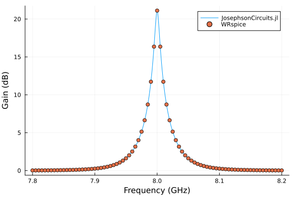
As detailed in [6], we find excellent agreement with Keysight ADS simulations and Fourier analysis of time domain simulation performed by WRSPICE.
Warning: this package is under heavy development and there will be breaking changes. We will keep the examples updated to ease the burden of any breaking changes.
To install the latest release of the package, install Julia using Juliaup, start Julia, and enter the following command:
using Pkg
Pkg.add("JosephsonCircuits")
To install the development version, start Julia and enter the command:
using Pkg
Pkg.add(name="JosephsonCircuits",rev="main")
To run the examples below, you will need to install Plots.jl using the command:
Pkg.add("Plots")
If you get errors when running the examples, please try installing the latest version of Julia and updating to the latest version of JosephsonCircuits.jl by running:
Pkg.update()
Then check that you are running the latest version of the package with:
Pkg.status()
Simulations of the linearized system can be effectively parallelized, so we suggest starting Julia with the number of threads equal to the number of physical cores. This can be done with the command line argument --threads or by setting the environmental variable JULIA_NUM_THREADS. See the Julia documentation for the more details. Verify you are using the desired number of threads by running:
Threads.nthreads()
For context, the simulation times reported for the examples below use 16 threads on an AMD Ryzen 9 9950X system running Linux.
The examples can be run in the command line (REPL) after starting Julia or you can run them in a Jupyter notebook with IJulia or in Visual Studio Code with the Julia extension.
Generate a netlist using circuit components including capacitors C, inductors L, Josephson junctions described by the Josephson inductance Lj, mutual inductors described by the mutual coupling coefficient K, and resistors R. See the SPICE netlist format, docstrings, and examples below for usage. Run the harmonic balance analysis using hbnlsolve to solve a nonlinear system at one operating point, hblinsolve to solve a linear (or linearized) system at one or more frequencies, or hbsolve to run both analyses. Add a question mark ? in front of a function to access the docstring. For example, type (don't copy-paste) the following to see the documentation for hbsolve:
?hbsolve
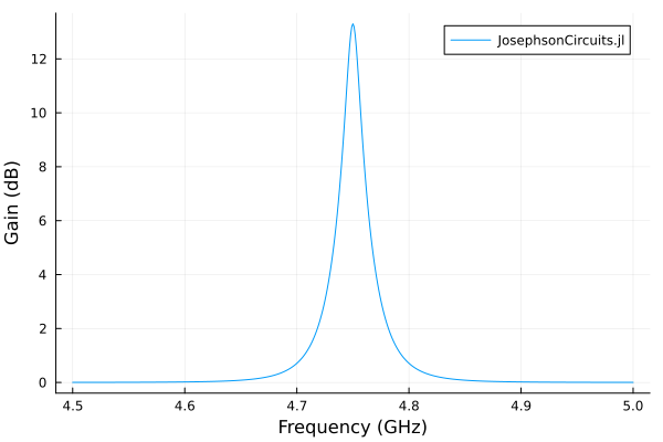
A driven nonlinear LC resonator.
using JosephsonCircuits
using Plots

@variables R Cc Lj Cj
circuit = [
    ("P1","1","0",1),
    ("R1","1","0",R),
    ("C1","1","2",Cc),
    ("Lj1","2","0",Lj),
    ("C2","2","0",Cj)]

circuitdefs = Dict(
    Lj =>1000.0e-12,
    Cc => 100.0e-15,
    Cj => 1000.0e-15,
    R => 50.0)

ws = 2*pi*(4.5:0.001:5.0)*1e9
wp = (2*pi*4.75001*1e9,)
Ip = 0.00565e-6
sources = [(mode=(1,),port=1,current=Ip)]
Npumpharmonics = (16,)
Nmodulationharmonics = (8,)

@time jpa = hbsolve(ws, wp, sources, Nmodulationharmonics,
    Npumpharmonics, circuit, circuitdefs)

plot(
    jpa.linearized.w/(2*pi*1e9),
    10*log10.(abs2.(
        jpa.linearized.S(
            outputmode=(0,),
            outputport=1,
            inputmode=(0,),
            inputport=1,
            freqindex=:
        ),
    )),
    label="JosephsonCircuits.jl",
    xlabel="Frequency (GHz)",
    ylabel="Gain (dB)",
)
0.001817 seconds (12.99 k allocations: 4.361 MiB)
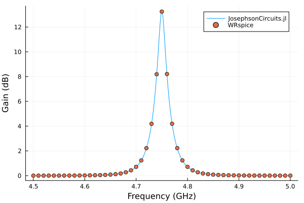
Compare with WRspice. Please note that on Linux you can install the XicTools_jll package which provides WRspice for x86_64. For other operating systems and platforms, you can install WRspice yourself and substitute XicTools_jll.wrspice() with JosephsonCircuits.wrspice_cmd() which will attempt to provide the path to your WRspice executable.
using XicTools_jll

wswrspice=2*pi*(4.5:0.01:5.0)*1e9
n = JosephsonCircuits.exportnetlist(circuit,circuitdefs);
input = JosephsonCircuits.wrspice_input_paramp(n.netlist,wswrspice,wp[1],2*Ip,(0,1),(0,1));

@time output = JosephsonCircuits.spice_run(input,XicTools_jll.wrspice());
S11,S21=JosephsonCircuits.wrspice_calcS_paramp(output,wswrspice,n.Nnodes);

plot!(wswrspice/(2*pi*1e9),10*log10.(abs2.(S11)),
    label="WRspice",
    seriestype=:scatter)
12.743245 seconds (32.66 k allocations: 499.263 MiB, 0.41% gc time)
Code
using JosephsonCircuits
using Plots
@variables R Cc Lj Cj
circuit = [
("P1","1","0",1),
("R1","1","0",R),
("C1","1","2",Cc),
("Lj1","2","0",Lj),
("C2","2","0",Cj)]
circuitdefs = Dict(
Lj =>1000.0e-12,
Cc => 100.0e-15,
Cj => 1000.0e-15,
R => 50.0)
ws = 2*pi*(4.5:0.001:5.0)*1e9
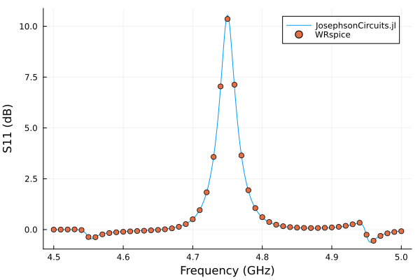
wp = (2*pi*4.65001*1e9,2*pi*4.85001*1e9)
Ip = 0.00565e-6*1.7
sources = [(mode=(1,0),port=1,current=Ip),(mode=(0,1),port=1,current=Ip)]
Npumpharmonics = (8,8)
Nmodulationharmonics = (8,8)
@time jpa = hbsolve(ws, wp, sources, Nmodulationharmonics,
Npumpharmonics, circuit, circuitdefs);
plot(
jpa.linearized.w/(2*pi*1e9),
10*log10.(abs2.(
jpa.linearized.S(
outputmode=(0,0),
outputport=1,
inputmode=(0,0),
inputport=1,
freqindex=:
),
)),
label="JosephsonCircuits.jl",
xlabel="Frequency (GHz)",
ylabel="S11 (dB)",
) 0.182720 seconds (12.70 k allocations: 713.087 MiB)
and compare with WRspice
Code
using XicTools_jll

wswrspice=2*pi*(4.5:0.01:5.0)*1e9
n = JosephsonCircuits.exportnetlist(circuit,circuitdefs);
input = JosephsonCircuits.wrspice_input_paramp(n.netlist,wswrspice,[wp[1],wp[2]],[2*Ip,2*Ip],(0,1),[(0,1),(0,1)]);

@time output = JosephsonCircuits.spice_run(input,XicTools_jll.wrspice());
S11,S21=JosephsonCircuits.wrspice_calcS_paramp(output,wswrspice,n.Nnodes,stepsperperiod = 50000);

plot!(wswrspice/(2*pi*1e9),10*log10.(abs2.(S11)),
    label="WRspice",
    seriestype=:scatter)
15.782862 seconds (32.80 k allocations: 509.192 MiB, 0.39% gc time)
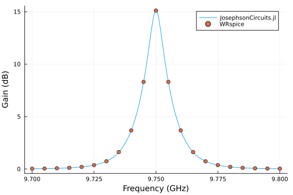
Circuit and parameters from here. Please note that three wave mixing (3WM) and flux-biasing are relatively untested, so you may encounter bugs. Please file issues or PRs.
Code
using JosephsonCircuits
using Plots

@variables R Cc Cj Lj Cr Lr Ll Ldc K Lg
circuit = [
    ("P1","1","0",1),
    ("R1","1","0",R),
    # a very large inductor so the DC node flux of this node isn't floating
    ("L0","1","0",Lg),
    ("C1","1","2",Cc),
    ("L1","2","3",Lr),
    ("C2","2","0",Cr),
    ("Lj1","3","0",Lj),
    ("Cj1","3","0",Cj),
    ("L2","3","4",Ll),
    ("Lj2","4","0",Lj),
    ("Cj2","4","0",Cj),
    ("L3","5","0",Ldc),
    ("K1","L2","L3",K),
    # a port with a very large resistor so we can apply the bias across the port
    ("P2","5","0",2),
    ("R2","5","0",1000.0),
]

circuitdefs = Dict(
    Lj =>219.63e-12,
    Lr =>0.4264e-9,
    Lg =>100.0e-9,
    Cc => 16.0e-15,
    Cj => 10.0e-15,
    Cr => 0.4e-12,
    R => 50.0,
    Ll => 34e-12,
    K => 0.999, # the inverse inductance matrix for K=1.0 diverges, so set K<1.0
    Ldc => 0.74e-12,
)

ws = 2*pi*(9.7:0.0001:9.8)*1e9
wp = (2*pi*19.50*1e9,)
Ip = 0.7e-6
Idc = 140.3e-6
# add the DC bias and pump to port 2
sourcespumpon = [(mode=(0,),port=2,current=Idc),(mode=(1,),port=2,current=Ip)]
Npumpharmonics = (16,)
Nmodulationharmonics = (8,)
@time jpapumpon = hbsolve(ws, wp, sourcespumpon, Nmodulationharmonics,
    Npumpharmonics, circuit, circuitdefs, dc = true, threewavemixing=true,fourwavemixing=true) # enable dc and three wave mixing


plot(
    jpapumpon.linearized.w/(2*pi*1e9),
    10*log10.(abs2.(
        jpapumpon.linearized.S(
            outputmode=(0,),
            outputport=1,
            inputmode=(0,),
            inputport=1,
            freqindex=:
        ),
    )),
    xlabel="Frequency (GHz)",
    ylabel="Gain (dB)",
    label="JosephsonCircuits.jl",
)
0.015623 seconds (22.07 k allocations: 80.082 MiB)
and compare with WRspice
Code
using XicTools_jll

# simulate the JPA in WRSPICE
wswrspice=2*pi*(9.7:0.005:9.8)*1e9
n = JosephsonCircuits.exportnetlist(circuit,circuitdefs);
input = JosephsonCircuits.wrspice_input_paramp(n.netlist,wswrspice,[0.0,wp[1]],[Idc,2*Ip],[(0,1)],[(0,5),(0,5)];trise=10e-9,tstop=600e-9);

# @time output = JosephsonCircuits.spice_run(input,JosephsonCircuits.wrspice_cmd());
@time output = JosephsonCircuits.spice_run(input,XicTools_jll.wrspice());
S11,S21=JosephsonCircuits.wrspice_calcS_paramp(output,wswrspice,n.Nnodes);

# plot the output
plot!(wswrspice/(2*pi*1e9),10*log10.(abs2.(S11)),
    label="WRspice",
    seriestype=:scatter)
283.557011 seconds (26.76 k allocations: 7.205 GiB, 0.66% gc time)
Simulate the JPA frequency as a function of DC bias current:
Code
ws = 2*pi*(8.0:0.01:11.0)*1e9
currentvals = (-20:0.1:20)*1e-5
outvals = zeros(Complex{Float64},length(ws),length(currentvals))
Ip=0.0

Npumpharmonics = (1,)
Nmodulationharmonics = (1,)

@time for (k,Idc) in enumerate(currentvals)
    sources = [
          (mode=(0,),port=2,current=Idc),
          (mode=(1,),port=2,current=Ip),
      ]
    sol = hbsolve(ws,wp,sources,Nmodulationharmonics, Npumpharmonics,
        circuit, circuitdefs;dc=true,threewavemixing=true,fourwavemixing=true)
    outvals[:,k]=sol.linearized.S((0,),1,(0,),1,:)
end

plot(
    currentvals/(1e-3),
    ws/(2*pi*1e9),
    10*log10.(abs2.(outvals)),
    seriestype=:heatmap,
    xlabel="bias current (mA)",
    ylabel="frequency (GHz)",
    title="S11 (dB), pump off",
)
0.219279 seconds (3.27 M allocations: 639.981 MiB, 20.84% gc time)
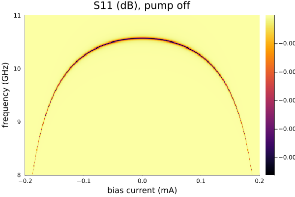
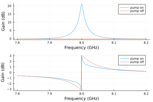
Circuit parameters from here. Notice that the resonance frequency is similar for pump-on and pump-off, indicating it is operating near the Kerr-free point.
Code
using JosephsonCircuits
using Plots

@variables R Cc Cj Lj Cr Lr Ll Ldc K Lg
alpha = 0.29
Z0 = 50
w0 = 2*pi*8e9
l=10e-3
circuit = [
    ("P1","1","0",1),
    ("R1","1","0",R),
    # a very large inductor so the DC node flux of this node isn't floating
    ("L0","1","0",Lg),
    ("C1","1","2",Cc),
    ("L1","2","3",Lr),
    ("C2","2","0",Cr),
    ("Lj1","3","0",Lj/alpha),
    ("Cj1","3","0",Cj/alpha),
    ("L2","3","4",Ll),
    ("Lj2","4","5",Lj),
    ("Cj2","4","5",Cj),
    ("Lj3","5","6",Lj),
    ("Cj3","5","6",Cj),
    ("Lj4","6","0",Lj),
    ("Cj4","6","0",Cj),
    ("L3","7","0",Ldc),
    ("K1","L2","L3",K),
    # a port with a very large resistor so we can apply the bias across the port
    ("P2","7","0",2),
    ("R2","7","0",1000.0),
]

circuitdefs = Dict(
    Lj => 60e-12,
    Cj => 10.0e-15,
    Lr =>0.4264e-9*1.25,
    Cr => 0.4e-12*1.25,
    Lg => 100.0e-9,
    Cc => 0.048e-12,
    R => 50.0,
    Ll => 34e-12,
    K => 0.999, # the inverse inductance matrix for K=1.0 diverges, so set K<1.0
    Ldc => 0.74e-12,
)

# ws = 2*pi*(9.7:0.0001:9.8)*1e9
# ws = 2*pi*(5.0:0.001:11)*1e9
ws = 2*pi*(7.8:0.001:8.2)*1e9
wp = (2*pi*16.00*1e9,)
Ip = 4.4e-6
# Idc = 140.3e-6
Idc = 0.000159
# add the DC bias and pump to port 2
sourcespumpon = [(mode=(0,),port=2,current=Idc),(mode=(1,),port=2,current=Ip)]
sourcespumpoff = [(mode=(0,),port=2,current=Idc),(mode=(1,),port=2,current=0.0)]
Npumpharmonics = (16,)
Nmodulationharmonics = (8,)
@time jpapumpon = hbsolve(ws, wp, sourcespumpon, Nmodulationharmonics,
    Npumpharmonics, circuit, circuitdefs, dc = true, threewavemixing=true,fourwavemixing=true) # enable dc and three wave mixing
@time jpapumpoff = hbsolve(ws, wp, sourcespumpoff, Nmodulationharmonics,
    Npumpharmonics, circuit, circuitdefs, dc = true, threewavemixing=true,fourwavemixing=true) # enable dc and three wave mixing

p1 = plot(
    jpapumpon.linearized.w/(2*pi*1e9),
    10*log10.(abs2.(
        jpapumpon.linearized.S(
            outputmode=(0,),
            outputport=1,
            inputmode=(0,),
            inputport=1,
            freqindex=:
        ),
    )),
    xlabel="Frequency (GHz)",
    ylabel="Gain (dB)",
    label="pump on",
)

plot!(
    jpapumpoff.linearized.w/(2*pi*1e9),
    10*log10.(abs2.(
        jpapumpoff.linearized.S(
            outputmode=(0,),
            outputport=1,
            inputmode=(0,),
            inputport=1,
            freqindex=:
        ),
    )),
    label="pump off",
)

p2 = plot(
    jpapumpon.linearized.w/(2*pi*1e9),
    angle.(
        jpapumpon.linearized.S(
            outputmode=(0,),
            outputport=1,
            inputmode=(0,),
            inputport=1,
            freqindex=:
        ),
    ),
    xlabel="Frequency (GHz)",
    ylabel="Gain (dB)",
    label="pump on",
)

plot!(
    jpapumpoff.linearized.w/(2*pi*1e9),
    angle.(
        jpapumpoff.linearized.S(
            outputmode=(0,),
            outputport=1,
            inputmode=(0,),
            inputport=1,
            freqindex=:
        ),
    ),
    label="pump off",
)
plot(p1,p2,layout=(2,1))
0.010345 seconds (16.74 k allocations: 40.025 MiB)
0.011252 seconds (16.68 k allocations: 39.985 MiB)
and compare with WRspice
Code
using XicTools_jll

# simulate the JPA in WRSPICE
wswrspice=2*pi*(7.8:0.005:8.2)*1e9
n = JosephsonCircuits.exportnetlist(circuit,circuitdefs);
input = JosephsonCircuits.wrspice_input_paramp(n.netlist,wswrspice,[0.0,wp[1]],[Idc,2*Ip],[(0,1)],[(0,7),(0,7)];trise=10e-9,tstop=600e-9);

@time output = JosephsonCircuits.spice_run(input,XicTools_jll.wrspice());
S11,S21=JosephsonCircuits.wrspice_calcS_paramp(output,wswrspice,n.Nnodes);

# plot the output
plot(
    jpapumpon.linearized.w/(2*pi*1e9),
    10*log10.(abs2.(
        jpapumpon.linearized.S(
            outputmode=(0,),
            outputport=1,
            inputmode=(0,),
            inputport=1,
            freqindex=:
        ),
    )),
    xlabel="Frequency (GHz)",
    ylabel="Gain (dB)",
    label="JosephsonCircuits.jl",
)

plot!(wswrspice/(2*pi*1e9),10*log10.(abs2.(S11)),
    label="WRspice",
    seriestype=:scatter)
2067.364975 seconds (149.73 k allocations: 29.873 GiB, 0.01% gc time)
Circuit parameters from here.
Code
using JosephsonCircuits
using Plots
@variables Rleft Rright Cg Lj Cj Cc Cr Lr
circuit = Tuple{String,String,String,Num}[]
# port on the input side
push!(circuit,("P$(1)_$(0)","1","0",1))
push!(circuit,("R$(1)_$(0)","1","0",Rleft))
Nj=2048
pmrpitch = 4
#first half cap to ground
push!(circuit,("C$(1)_$(0)","1","0",Cg/2))
#middle caps and jj's
push!(circuit,("Lj$(1)_$(2)","1","2",Lj))
push!(circuit,("C$(1)_$(2)","1","2",Cj))
j=2
for i = 2:Nj-1
if mod(i,pmrpitch) == pmrpitch÷2
# make the jj cell with modified capacitance to ground
push!(circuit,("C$(j)_$(0)","$(j)","$(0)",Cg-Cc))
push!(circuit,("Lj$(j)_$(j+2)","$(j)","$(j+2)",Lj))
push!(circuit,("C$(j)_$(j+2)","$(j)","$(j+2)",Cj))
#make the pmr
push!(circuit,("C$(j)_$(j+1)","$(j)","$(j+1)",Cc))
push!(circuit,("C$(j+1)_$(0)","$(j+1)","$(0)",Cr))
push!(circuit,("L$(j+1)_$(0)","$(j+1)","$(0)",Lr))
# increment the index
j+=1
else
push!(circuit,("C$(j)_$(0)","$(j)","$(0)",Cg))
push!(circuit,("Lj$(j)_$(j+1)","$(j)","$(j+1)",Lj))
push!(circuit,("C$(j)_$(j+1)","$(j)","$(j+1)",Cj))
end
# increment the index
j+=1
end
#last jj
push!(circuit,("C$(j)_$(0)","$(j)","$(0)",Cg/2))
push!(circuit,("R$(j)_$(0)","$(j)","$(0)",Rright))
# port on the output side
push!(circuit,("P$(j)_$(0)","$(j)","$(0)",2))
circuitdefs = Dict(
Lj => IctoLj(3.4e-6),
Cg => 45.0e-15,
Cc => 30.0e-15,
Cr => 2.8153e-12,
Lr => 1.70e-10,
Cj => 55e-15,
Rleft => 50.0,
Rright => 50.0,
)
ws=2*pi*(1.0:0.1:14)*1e9
wp=(2*pi*7.12*1e9,)
Ip=1.85e-6
sources = [(mode=(1,),port=1,current=Ip)]
Npumpharmonics = (20,)
Nmodulationharmonics = (10,)
@time rpm = hbsolve(ws, wp, sources, Nmodulationharmonics,
Npumpharmonics, circuit, circuitdefs)
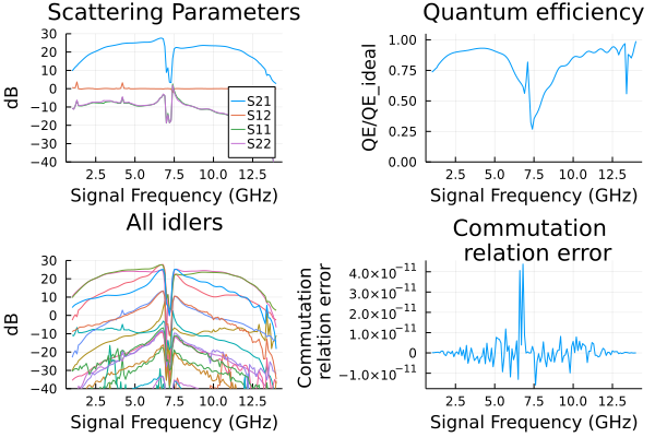
p1=plot(ws/(2*pi*1e9),
10*log10.(abs2.(rpm.linearized.S(
outputmode=(0,),
outputport=2,
inputmode=(0,),
inputport=1,
freqindex=:),
)),
ylim=(-40,30),label="S21",
xlabel="Signal Frequency (GHz)",
legend=:bottomright,
title="Scattering Parameters",
ylabel="dB")
plot!(ws/(2*pi*1e9),
10*log10.(abs2.(rpm.linearized.S((0,),1,(0,),2,:))),
label="S12",
)
plot!(ws/(2*pi*1e9),
10*log10.(abs2.(rpm.linearized.S((0,),1,(0,),1,:))),
label="S11",
)
plot!(ws/(2*pi*1e9),
10*log10.(abs2.(rpm.linearized.S((0,),2,(0,),2,:))),
label="S22",
)
p2=plot(ws/(2*pi*1e9),
rpm.linearized.QE((0,),2,(0,),1,:)./rpm.linearized.QEideal((0,),2,(0,),1,:),
ylim=(0,1.05),
title="Quantum efficiency",legend=false,
ylabel="QE/QE_ideal",xlabel="Signal Frequency (GHz)");
p3=plot(ws/(2*pi*1e9),
10*log10.(abs2.(rpm.linearized.S(:,2,(0,),1,:)')),
ylim=(-40,30),
xlabel="Signal Frequency (GHz)",
legend=false,
title="All idlers",
ylabel="dB")
p4=plot(ws/(2*pi*1e9),
1 .- rpm.linearized.CM((0,),2,:),
legend=false,title="Commutation \n relation error",
ylabel="Commutation \n relation error",xlabel="Signal Frequency (GHz)");
plot(p1, p2, p3, p4, layout = (2, 2)) 2.959010 seconds (257.75 k allocations: 2.392 GiB, 0.21% gc time)
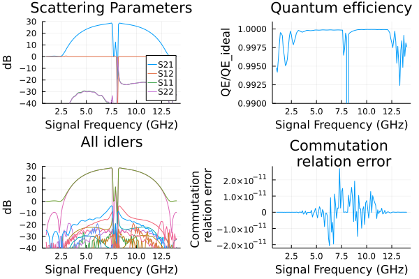
Circuit parameters from here.
Code
using JosephsonCircuits
using Plots

@variables Rleft Rright Lj Cg Cc Cr Lr Cj

weightwidth = 745
weight = (n,Nnodes,weightwidth) -> exp(-(n - Nnodes/2)^2/(weightwidth)^2)
Nj=2000
pmrpitch = 8

# define the circuit components
circuit = Tuple{String,String,String,Num}[]

# port on the left side
push!(circuit,("P$(1)_$(0)","1","0",1))
push!(circuit,("R$(1)_$(0)","1","0",Rleft))

#first half cap to ground
push!(circuit,("C$(1)_$(0)","1","0",Cg/2*weight(1-0.5,Nj,weightwidth)))
#middle caps and jj's
push!(circuit,("Lj$(1)_$(2)","1","2",Lj*weight(1,Nj,weightwidth)))
push!(circuit,("C$(1)_$(2)","1","2",Cj/weight(1,Nj,weightwidth)))

j=2
for i = 2:Nj-1

    if mod(i,pmrpitch) == pmrpitch÷2

        # make the jj cell with modified capacitance to ground
        push!(circuit,("C$(j)_$(0)","$(j)","$(0)",(Cg-Cc)*weight(i-0.5,Nj,weightwidth)))
        push!(circuit,("Lj$(j)_$(j+2)","$(j)","$(j+2)",Lj*weight(i,Nj,weightwidth)))

        push!(circuit,("C$(j)_$(j+2)","$(j)","$(j+2)",Cj/weight(i,Nj,weightwidth)))

        #make the pmr
        push!(circuit,("C$(j)_$(j+1)","$(j)","$(j+1)",Cc*weight(i-0.5,Nj,weightwidth)))
        push!(circuit,("C$(j+1)_$(0)","$(j+1)","$(0)",Cr))
        push!(circuit,("L$(j+1)_$(0)","$(j+1)","$(0)",Lr))

        # increment the index
        j+=1
    else
        push!(circuit,("C$(j)_$(0)","$(j)","$(0)",Cg*weight(i-0.5,Nj,weightwidth)))
        push!(circuit,("Lj$(j)_$(j+1)","$(j)","$(j+1)",Lj*weight(i,Nj,weightwidth)))
        push!(circuit,("C$(j)_$(j+1)","$(j)","$(j+1)",Cj/weight(i,Nj,weightwidth)))
    end

    # increment the index
    j+=1

end

#last jj
push!(circuit,("C$(j)_$(0)","$(j)","$(0)",Cg/2*weight(Nj-0.5,Nj,weightwidth)))
push!(circuit,("R$(j)_$(0)","$(j)","$(0)",Rright))
push!(circuit,("P$(j)_$(0)","$(j)","$(0)",2))

circuitdefs = Dict(
    Rleft => 50.0,
    Rright => 50.0,
    Lj => IctoLj(1.75e-6),
    Cg => 76.6e-15,
    Cc => 40.0e-15,
    Cr =>  1.533e-12,
    Lr => 2.47e-10,
    Cj => 40e-15,
)

ws=2*pi*(1.0:0.1:14)*1e9
wp=(2*pi*7.9*1e9,)
Ip=1.1e-6
sources = [(mode=(1,),port=1,current=Ip)]
Npumpharmonics = (20,)
Nmodulationharmonics = (10,)

@time floquet = hbsolve(ws, wp, sources, Nmodulationharmonics,
    Npumpharmonics, circuit, circuitdefs)

p1=plot(ws/(2*pi*1e9),
    10*log10.(abs2.(floquet.linearized.S((0,),2,(0,),1,:))),
    ylim=(-40,30),label="S21",
    xlabel="Signal Frequency (GHz)",
    legend=:bottomright,
    title="Scattering Parameters",
    ylabel="dB")

plot!(ws/(2*pi*1e9),
    10*log10.(abs2.(floquet.linearized.S((0,),1,(0,),2,:))),
    label="S12",
    )

plot!(ws/(2*pi*1e9),
    10*log10.(abs2.(floquet.linearized.S((0,),1,(0,),1,:))),
    label="S11",
    )

plot!(ws/(2*pi*1e9),
    10*log10.(abs2.(floquet.linearized.S((0,),2,(0,),2,:))),
    label="S22",
    )

p2=plot(ws/(2*pi*1e9),
    floquet.linearized.QE((0,),2,(0,),1,:)./floquet.linearized.QEideal((0,),2,(0,),1,:),
    ylim=(0.99,1.001),
    title="Quantum efficiency",legend=false,
    ylabel="QE/QE_ideal",xlabel="Signal Frequency (GHz)");

p3=plot(ws/(2*pi*1e9),
    10*log10.(abs2.(floquet.linearized.S(:,2,(0,),1,:)')),
    ylim=(-40,30),label="S21",
    xlabel="Signal Frequency (GHz)",
    legend=false,
    title="All idlers",
    ylabel="dB")


p4=plot(ws/(2*pi*1e9),
    1 .- floquet.linearized.CM((0,),2,:),
    legend=false,title="Commutation \n relation error",
    ylabel="Commutation \n relation error",xlabel="Signal Frequency (GHz)");

plot(p1, p2, p3,p4,layout = (2, 2))
2.079267 seconds (456.63 k allocations: 1.997 GiB, 0.48% gc time)
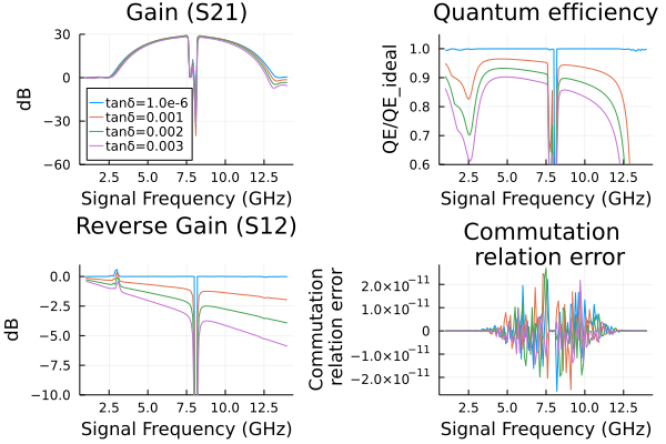
Dissipation due to capacitors with dielectric loss, parameterized by a loss tangent. Run the above code block to define the circuit then run the following:
Code
results = []
tandeltas = [1.0e-6,1.0e-3, 2.0e-3, 3.0e-3]
for tandelta in tandeltas
    circuitdefs = Dict(
        Rleft => 50,
        Rright => 50,
        Lj => IctoLj(1.75e-6),
        Cg => 76.6e-15/(1+im*tandelta),
        Cc => 40.0e-15/(1+im*tandelta),
        Cr => 1.533e-12/(1+im*tandelta),
        Lr => 2.47e-10,
        Cj => 40e-15,
    )
    wp=(2*pi*7.9*1e9,)
    ws=2*pi*(1.0:0.1:14)*1e9
    Ip=1.1e-6*(1+125*tandelta)
    sources = [(mode=(1,),port=1,current=Ip)]
    Npumpharmonics = (20,)
    Nmodulationharmonics = (10,)
    @time floquet = hbsolve(ws, wp, sources, Nmodulationharmonics,
        Npumpharmonics, circuit, circuitdefs)
    push!(results,floquet)
end

p1 = plot(title="Gain (S21)")
for i = 1:length(results)
        plot!(ws/(2*pi*1e9),
            10*log10.(abs2.(results[i].linearized.S((0,),2,(0,),1,:))),
            ylim=(-60,30),label="tanδ=$(tandeltas[i])",
            legend=:bottomleft,
            xlabel="Signal Frequency (GHz)",ylabel="dB")
end

p2 = plot(title="Quantum Efficiency")
for i = 1:length(results)
        plot!(ws/(2*pi*1e9),
            results[i].linearized.QE((0,),2,(0,),1,:)./results[i].linearized.QEideal((0,),2,(0,),1,:),
            ylim=(0.6,1.05),legend=false,
            title="Quantum efficiency",
            ylabel="QE/QE_ideal",xlabel="Signal Frequency (GHz)")
end

p3 = plot(title="Reverse Gain (S12)")
for i = 1:length(results)
        plot!(ws/(2*pi*1e9),
            10*log10.(abs2.(results[i].linearized.S((0,),1,(0,),2,:))),
            ylim=(-10,1),legend=false,
            xlabel="Signal Frequency (GHz)",ylabel="dB")
end

p4 = plot(title="Commutation \n relation error")
for i = 1:length(results)
        plot!(ws/(2*pi*1e9),
            1 .- results[i].linearized.CM((0,),2,:),
            legend=false,
            ylabel="Commutation\n relation error",xlabel="Signal Frequency (GHz)")
end

plot(p1, p2, p3,p4,layout = (2, 2))
3.815835 seconds (470.00 k allocations: 2.303 GiB, 0.22% gc time)
3.800166 seconds (470.59 k allocations: 2.310 GiB, 0.29% gc time)
3.824690 seconds (470.75 k allocations: 2.317 GiB, 0.19% gc time)
3.838721 seconds (470.75 k allocations: 2.317 GiB, 0.18% gc time)
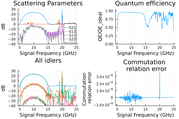
Circuit and parameters from here. Please note that three wave mixing (3WM) and flux-biasing are relatively untested, so you may encounter bugs. Please file issues or PRs.
Code
using JosephsonCircuits
using Plots

const magnetic_flux_quantum = 2.0678338484619295e-15
const reduced_magnetic_flux_quantum = magnetic_flux_quantum / (2*pi)

@variables Rport C Cj Lj Lpump Cpump kappa Lg Lsmall


# From Section V. POSSIBLE CIRCUIT DESIGN
cutoff_frequency = 46e9 # [Hz]
transmission_line_impedance = 50.0

capacitance = 1 / (2 * pi * cutoff_frequency * transmission_line_impedance) # equation (51) [H]
junction_inductance = transmission_line_impedance / (2 * pi * cutoff_frequency) # L = L', equation (52) [F]
critical_current = reduced_magnetic_flux_quantum / junction_inductance

critical_current_density = 3e6 # Typical value mentioned in paper [A/m^2]
jj_area = critical_current / critical_current_density # [m^2]
jj_cap_density = 50 * 1e-15 / (1e-6)^2 # Typical [F/m^2]
jj_capacitance = jj_cap_density * jj_area

nr_cells = 500
modulation_parameter = 0.06

coupling = 0.02 # = M / L', equation (8)
mutual_inductance = coupling * junction_inductance
# Add small linear inductance in dc-SQUID loop to couple pump line inductance with
linear_squid_loop_inductance = mutual_inductance^2 / junction_inductance

# in order to reduce critical current of dc squid to critical current of junction
optimal_dc_flux = magnetic_flux_quantum / 3
Idc = optimal_dc_flux / mutual_inductance
Ip = modulation_parameter * Idc

pump_line_inductance = 1.1 * junction_inductance

pump_frequency = 20e9 # [Hz]
frequency_detuning = range(-0.5, 1.5, 500)
signal_frequency = pump_frequency / 2 .* (frequency_detuning .+ 1)

circuit = Tuple{String,String,String,Num}[]
entry = (elem, n1, n2, value) -> push!(circuit, ("$(elem)$(n1)_$(n2)", "$n1", "$n2", value))

function build_circuit()
    node = 1

    node_p1 = node # P1: Start of transmission line
    entry("P", node_p1, 0, 1)
    entry("R", node_p1, 0, Rport)

    node_p3 = node+1 # P3: Start of pump line
    entry("P", node_p3, 0, 3)
    entry("R", node_p3, 0, Rport)

    for cell_index in 1:nr_cells
        if cell_index == 1
            entry("C", node, 0, C/2)
        else
            entry("C", node, 0, C)
        end
        entry("Lj_a", node, node+3, Lj)
        entry("Cj_a", node, node+3, Cj)
        entry("L", node, node+2, Lsmall)
        entry("Lj_b", node+2, node+3, Lj)
        entry("Cj_b", node+2, node+3, Cj)

        entry("L", node+1, node+4, Lpump)
        if cell_index == 1
            entry("C", node+1, 0, Cpump/2)
        else
            entry("C", node+1, 0, Cpump)
        end
        push!(circuit, ("K$(node)", "L$(node)_$(node+2)", "L$(node+1)_$(node+4)", kappa))

        node += 3
    end

    entry("C", node, 0, C/2)
    entry("P", node, 0, 2) # P2: End of transmission line
    entry("R", node, 0, Rport)

    entry("C", node+1, 0, Cpump/2)
    entry("P", node+1, 0, 4) # P4: End of pump line
    entry("R", node+1, 0, Rport)
    entry("L", node+1, 0, Lg)

end

build_circuit()

circuitdefs = Dict(
    kappa => 0.999,
    Lg => 20.0e-9, # inductance to ground, required for solver
    Rport => 50.0,
    C => capacitance,
    Lj => junction_inductance,
    Lpump => pump_line_inductance,
    Cpump => pump_line_inductance / transmission_line_impedance^2,
    Lsmall => linear_squid_loop_inductance,
    Cj => jj_capacitance,
)

ws = 2*pi*signal_frequency
wp = (2*pi*pump_frequency,)

# add the DC bias and pump to port 3
sourcespumpon = [(mode=(0,),port=3,current=Idc),(mode=(1,),port=3,current=Ip)]
Npumpharmonics = (8,)
Nmodulationharmonics = (4,)
@time sol = hbsolve(ws, wp, sourcespumpon, Nmodulationharmonics,
    Npumpharmonics, circuit, circuitdefs;
    dc = true, threewavemixing=true,fourwavemixing=true,
    switchofflinesearchtol=0.0,alphamin=1e-7,iterations=200) # enable dc and three wave mixing

p1=plot(sol.linearized.w/(2*pi*1e9),
    10*log10.(abs2.(sol.linearized.S(
            outputmode=(0,),
            outputport=2,
            inputmode=(0,),
            inputport=1,
            freqindex=:),
    )),
    ylim=(-40,30),label="S21",
    xlabel="Signal Frequency (GHz)",
    legend=:bottomright,
    title="Scattering Parameters",
    ylabel="dB");

plot!(sol.linearized.w/(2*pi*1e9),
    10*log10.(abs2.(sol.linearized.S((0,),1,(0,),2,:))),
    label="S12",
    );

plot!(sol.linearized.w/(2*pi*1e9),
    10*log10.(abs2.(sol.linearized.S((0,),1,(0,),1,:))),
    label="S11",
    );

plot!(sol.linearized.w/(2*pi*1e9),
    10*log10.(abs2.(sol.linearized.S((0,),2,(0,),2,:))),
    label="S22",
    );

p2=plot(sol.linearized.w/(2*pi*1e9),
    sol.linearized.QE((0,),2,(0,),1,:)./sol.linearized.QEideal((0,),2,(0,),1,:),
    ylim=(0,1.05),
    title="Quantum efficiency",legend=false,
    ylabel="QE/QE_ideal",xlabel="Signal Frequency (GHz)");

p3=plot(sol.linearized.w/(2*pi*1e9),
    10*log10.(abs2.(sol.linearized.S(:,2,(0,),1,:)')),
    ylim=(-40,30),
    xlabel="Signal Frequency (GHz)",
    legend=false,
    title="All idlers",
    ylabel="dB");

p4=plot(sol.linearized.w/(2*pi*1e9),
    1 .- sol.linearized.CM((0,),2,:),
    legend=false,title="Commutation \n relation error",
    ylabel="Commutation \n relation error",xlabel="Signal Frequency (GHz)");

plot(p1, p2, p3, p4, layout = (2, 2))
28.342059 seconds (1.59 M allocations: 1.637 GiB, 0.35% gc time)
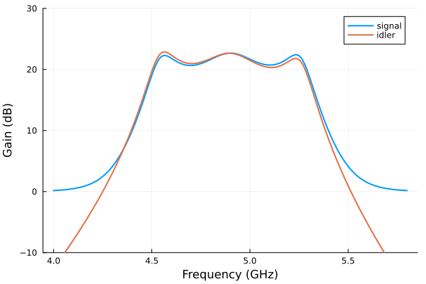
Circuit parameters of the lumped-element snake amplifier (LESA) from here.
Code
Utility functions
using JosephsonCircuits, Plots

function calc_Lsnake(N,L1,L2,LJ,delta0)
   return N/2*((L1+L2)*LJ+L1*L2*cos(delta0))/(LJ+(4*L1+L2)*cos(delta0))
end

"""
    add_snake!(circuit,start_node,skip_nodes,L1,L2,Lj,Nstages)

Add a `snake` a tunable inductor made of two rf-SQUID arrays
in parallel as detailed in arXiv:2209.07757 and PhysRevLett.109.137003
to the netlist contained in `circuit`. See also [`add_snake_squid!`](@ref).

            <-----------Nstages------ ... -->
             stage
            <----->start_node+skip_nodes+2
start_node o--Lj--o--L2--o--Lj- ... -o--L2--o
           |      |      |           |      |
           L1     L1     L1          L1     L1
           |      |      |           |      |
           o--L2--o--Lj--o--L2- ...  o--Lj--o end_node
start_node     start_node
+skip_nodes+1  +skip_nodes+3

# Arguments
- `circuit`: Vector of tuples containing the netlist.
- `start_node`: The first node of the transmission line.
- `skip_nodes`: The number of nodes to skip before the device.
- `L1`: Inductor of the inductance from upper to lower.
- `L2`: Inductance of the upper/lower inductor.
- `Lj`: Inductance of the Josephson junction.
- `Nstages`: The number of stages (JJs) in the snake.

# Returns
- `end_node`: The last node of the transmission line.
- `skip_nodes`: The number of nodes to skip after end_node. Always 0.
"""
function add_snake!(circuit,start_node,skip_nodes,L1,L2,Lj,Nstages)
    # add examples, fix behavior for skip_nodes
    # check that returned end_node skip_node behavior correct

    # add the SNAKE
    j=start_node+skip_nodes
    # add the first stage outside of the loop
    # so we can keep the same pattern in the array

    # L1 linear inductor at the start of the stage
    push!(circuit,("L$(start_node)_$(j+1)","$(start_node)","$(j+1)",L1))
    # the L1 linear inductor at the end of the stage
    push!(circuit,("L$(j+2)_$(j+3)","$(j+2)","$(j+3)",L1))
    # the JJ
    push!(circuit,("Lj$(start_node)_$(j+2)","$(start_node)","$(j+2)",Lj))
    # then L2
    push!(circuit,("L$(j+1)_$(j+3)","$(j+1)","$(j+3)",L2))
    # increase the current node number by 2
    # since each cell adds 2 nodes
    j+=2
    for i in 2:Nstages
        # the L1 linear inductor at the end of the stage
        push!(circuit,("L$(j+2)_$(j+3)","$(j+2)","$(j+3)",L1))

        # JJ and L1 swap places
        if !iszero(mod(i,2)) # first cell and every odd cell
            # JJ is first
            push!(circuit,("Lj$(j)_$(j+2)","$(j)","$(j+2)",Lj))
            # then L2
            push!(circuit,("L$(j+1)_$(j+3)","$(j+1)","$(j+3)",L2))
        else
            # inductor is first
            push!(circuit,("L$(j)_$(j+2)","$(j)","$(j+2)",L2))
            # then JJ
            push!(circuit,("Lj$(j+1)_$(j+3)","$(j+1)","$(j+3)",Lj))
        end
        # increase the current node number by 2
        # since each cell adds 2 nodes
        j+=2
    end
    skip_nodes = 0
    end_node = j+1
    return (end_node,skip_nodes)
end

"""
    add_snake_squid!(circuit,start_node,skip_nodes,L1,L2,L3,Lj,Lb,K,R,Nstages)

Add a SQUID made of four `snakes` (tunable inductors made of two rf-SQUID arrays
in parallel) as detailed in arXiv:2209.07757 and PhysRevLett.109.137003
to the netlist contained in `circuit`. See also [`add_snake!`](@ref).

     start_node o
                |
                |
---snake-------------------snake---
|                 -               |
L3               ---              L3
|                 |               |
---snake--|       R     |--snake---
          |       |     |
          |  Port o     |
          |       |     |
          Lb  K   Lb    |
          |       |     |
          |       Lb  K Lb
          |       |     |
         ---     ---   ---
          -       -     -

# Arguments
- `circuit`: Vector of tuples containing the netlist.
- `start_node`: The first node of the transmission line.
- `skip_nodes`: The number of nodes to skip before the device.
- `L1`: Inductance of the inductor from upper to lower
    branch of snake.
- `L2`: Inductance of the upper/lower inductor.
- `L3`: Inductance in series between the snakes.
- `Lj`: Inductance of the Josephson junction.
- `Lb`: Inductance of inductors on the bias lines.
- `K`: Mutual inductance between the bias line to the SQUID
- `R`: Resistance of the bias port.
- `Nstages`: The number of stages (JJs) in the snake. The
    snake SQUID will have 4*Nstages JJs.

# Returns
- `end_node`: The last node of the transmission line.
- `skip_nodes`: The number of nodes to skip after end_node. Always 0.
"""
function add_snake_squid!(circuit,start_node,skip_nodes,L1,L2,L3,Lj,Lb,K,R,Nstages)
    # add examples, fix behavior for skip_nodes
    # check that returned end_node skip_node behavior correct

    # first snake
    # start_node = 1
    # skip_nodes = 0
    end_node,skip_nodes = add_snake!(circuit,start_node,skip_nodes,L1,L2,Lj,Nstages)
    j = end_node

    # linear inductor in between the snakes
    push!(circuit,("L$(j)_$(j+1)","$(j)","$(j+1)",L3))
    j+=1

    # second snake
    start_node = j
    skip_nodes = 0
    end_node,skip_nodes = add_snake!(circuit,start_node,skip_nodes,L1,L2,Lj,Nstages)
    j = end_node

    # add the coupling to bias inductors Lb1
    push!(circuit,("L$(j)_$(0)","$(j)","0",Lb))
    push!(circuit,("Kb1","L$(j)_$(0)","Lb1",K))
    j+=1

    # add the second arm of the snake
    # third snake
    start_node = 1
    skip_nodes = j-start_node-1
    end_node,skip_nodes = add_snake!(circuit,start_node,skip_nodes,L1,L2,Lj,Nstages)
    j = end_node

    # linear inductor in between the snakes
    push!(circuit,("L$(j)_$(j+1)","$(j)","$(j+1)",L3))
    j+=1

    # fourth snake
    start_node = j
    skip_nodes = 0
    end_node,skip_nodes = add_snake!(circuit,start_node,skip_nodes,L1,L2,Lj,Nstages)
    j = end_node

    # add the coupling to bias inductors Lb2
    push!(circuit,("L$(j)_$(0)","$(j)","0",Lb))
    push!(circuit,("Kb2","L$(j)_$(0)","Lb2",K))
    j+=1

    # bias across this port
    push!(circuit,("P2","$(j)","$(0)",2))
    push!(circuit,("R$(j)_$(0)","$(j)","$(0)",R))

    # add the two bias inductors
    push!(circuit,("Lb1","$(j)","$(j+1)",Lb))
    push!(circuit,("Lb2","$(j+1)","0",Lb))

    end_node = j+1
    skip_nodes = 0
    return (end_node,skip_nodes)

end

"""
    add_tline!(circuit,start_node,skip_nodes,theta,w0,wc,Z0)

Add an LC ladder that approximates a transmission line to the netlist
contained in `circuit`. The transmission line starts and ends with
half an inductor.

start_node       start_node+skip_nodes+1
          o--L/2--o- ... --L--- ... ---L/2--o
                  |           |
                  C           C
                  |           |
          o--------- ... ------- ... -------o
                          Ncells-1
# Arguments
- `circuit`: Vector of tuples containing the netlist.
- `start_node`: The first node of the transmission line.
- `skip_nodes`: The number of nodes to skip before the second
    node of the transmission line.
- `theta`: The phase angle of the transmission line at frequency w0.
- `Z0`: The characteristic impedance.
- `w0`: The frequency at which the phase angle is defined.
- `wc`: The cutoff frequency of the LC ladder. This should likely
    be much higher than w0. This determines the number of cells
    in the transmission line.

# Returns
- `end_node`: The last node of the transmission line.
- `skip_nodes`: The number of nodes to skip after end_node. Always 0.
"""
function add_tline!(circuit,start_node,skip_nodes,theta,w0,wc,Z0)
    # add examples, fix behavior for skip_nodes
    # check that returned end_node skip_node behavior correct

    # based on the cutoff frequency, operating frequency, and phase shift
    # estimate the number of cells required.
    # round up
    Ncells = ceil(theta*wc/(2*w0))

    # based on the rounded number of cells, revise the cutoff frequency
    # and compute the capacitance and inductance per unit cell
    wc = Ncells*2*w0/theta

    # inductance and capacitance per cell
    L = 2*Z0/wc
    C = 2/(wc*Z0)


    j = start_node
    for i = 1:Ncells
        if i == 1
            # start with half an inductor
            push!(circuit,("L$(j)_$(j+1)","$(j)","$(j+1)",L/2))
            j+=1
        end
        push!(circuit,("C$(j)_$(0)","$(j)","$(0)",C))
        if i == Ncells
            # end with half an inductor
            push!(circuit,("L$(j)_$(j+1)","$(j)","$(j+1)",L/2))
        else
            push!(circuit,("L$(j)_$(j+1)","$(j)","$(j+1)",L))
        end
        # increment the index
        j+=1
    end
    end_node = j
    skip_nodes = 0
    return (end_node,skip_nodes)
end
LESA simulation
@variables R Lj L1 L2 L3 Lb K Lg C1 PLCC PLCL L22 C6 C7
Nstages_snake = 10

circuit = Tuple{String,String,String,Num}[]


# add X1, a snake squid
start_node = 1
skip_nodes = 0
end_node, skip_nodes = add_snake_squid!(circuit,start_node,skip_nodes,L1,L2,L3,Lj,Lb,K,R,Nstages_snake)
j = end_node
# and add C1, a capacitor to ground
push!(circuit,("C$(start_node)_$(0)","$(start_node)","$(0)",C1))
# add C6, a series capacitor
push!(circuit,("C$(start_node)_$(j+1)","$(start_node)","$(j+1)",C6))
j+=1

# add PLC1, a parallel LC capacitor to ground
push!(circuit,("C$(j)_$(0)","$(j)","$(0)",PLCC))
push!(circuit,("L$(j)_$(0)","$(j)","$(0)",PLCL))
# add C7, a series capacitor
push!(circuit,("C$(j)_$(j+1)","$(j)","$(j+1)",C7))
j+=1

# end
Z0 = 50.0
w0 = 2*pi*4.9e9
wc = 2*pi*150e9
theta = 32.6*pi/180
start_node = j
skip_nodes = 0
end_node, skip_nodes = add_tline!(circuit,start_node,skip_nodes,theta,w0,wc,Z0)
j = end_node

push!(circuit,("L$(j)_$(0)","$(j)","$(0)",L22))
push!(circuit,("P1","$(j)","$(0)",1))
push!(circuit,("R1","$(j)","$(0)",R))

circuitdefs = Dict(
    Lj => JosephsonCircuits.IctoLj(16e-6),
    L1 => 2.6e-12,
    L2 => 8.0e-12,
    L3 => 5e-12,
    Lg => 100.0e-9,
    L22 => 1.320e-9,
    C1 => 6.607e-12,
    C6 => 0.743e-12,
    C7 => 0.265e-12,
    PLCC => 0.654e-12,
    PLCL => 0.650e-9,
    R => 50.0,
    Lb => 60e-12,
    K => 0.5*50/sqrt(60*60),
)

# ws = 2*pi*(1:0.01:10.0)*1e9
ws = 2*pi*(4.0:0.01:5.8)*1e9
wp = (2*pi*9.8001*1e9,)
Ip = 0.247e-3
Idc = 0.686e-3
# add the DC bias and pump to port 2
sourcespumpon = [(mode=(0,),port=2,current=Idc),(mode=(1,),port=2,current=Ip)]
Npumpharmonics = (8,)
Nmodulationharmonics = (4,)
@time sol = hbsolve(ws, wp, sourcespumpon, Nmodulationharmonics,
    Npumpharmonics, circuit, circuitdefs, dc = true, threewavemixing=true,fourwavemixing=true,
        switchofflinesearchtol=0.0,alphamin=1e-7,iterations=200,
)

plot(
    sol.linearized.w/(2*pi*1e9),
    10*log10.(abs2.(
        sol.linearized.S(
            outputmode=(0,),
            outputport=1,
            inputmode=(0,),
            inputport=1,
            freqindex=:
        ),
    )),
    xlabel="Frequency (GHz)",
    ylabel="Gain (dB)",
    label="signal",
    linewidth=2,
    ylim=(-10,30),
#     ylim=(19,22),
#     xlim=(4.69,4.71),
)

plot!(
    sol.linearized.w/(2*pi*1e9),
    10*log10.(abs2.(
        sol.linearized.S(
            outputmode=(-1,),
            outputport=1,
            inputmode=(0,),
            inputport=1,
            freqindex=:
        ).*sqrt.(abs.((wp.-sol.linearized.w)./sol.linearized.w)), # convert from photon number to power
    )),
    linewidth=2,
    xlabel="Frequency (GHz)",
    ylabel="Gain (dB)",
    label="idler",
)
0.081631 seconds (34.78 k allocations: 67.609 MiB, 48.06% gc time)
We welcome contributions in the form of issues/bug reports or pull requests. This project uses the MIT open source license. You retain the copyright to any code you contribute.
- Andrew J. Kerman "Efficient numerical simulation of complex Josephson quantum circuits" arXiv:2010.14929 (2020)
- Jiří Vlach and Kishore Singhal "Computer Methods for Circuit Analysis and Design" 2nd edition, Springer New York, NY (1993)
- Stephen A. Maas "Nonlinear Microwave and RF Circuits" 2nd edition, Artech House (1997)
- José Carlos Pedro, David E. Root, Jianjun Xu, and Luís Cótimos Nunes. "Nonlinear Circuit Simulation and Modeling: Fundamentals for Microwave Design" The Cambridge RF and Microwave Engineering Series, Cambridge University Press (2018)
- David E. Root, Jan Verspecht, Jason Horn, and Mihai Marcu. "X-Parameters: Characterization, Modeling, and Design of Nonlinear RF and Microwave Components" The Cambridge RF and microwave engineering series, Cambridge University Press (2013)
- Kaidong Peng, Rick Poore, Philip Krantz, David E. Root, and Kevin P. O'Brien "X-parameter based design and simulation of Josephson traveling-wave parametric amplifiers for quantum computing applications" IEEE International Conference on Quantum Computing & Engineering (QCE22) (2022)
The motivation for developing this package is to simulate the gain and noise performance of ultra low noise amplifiers for quantum computing applications such as the Josephson traveling-wave parametric amplifier, which have thousands of linear and nonlinear circuit elements.
We prioritize speed (including compile time and time to first use), simplicity, and scalability.
- Design optimization.
- More nonlinear components such as kinetic inductors.
- Time domain simulations.
- Xyce.jl provides a wrapper for Xyce, the open source parallel circuit simulator from Sandia National Laboratories which can perform time domain and harmonic balance method simulations.
- NgSpice.jl and LTspice.jl provide wrappers for NgSpice and LTspice, respectively.
- ModelingToolkit.jl supports time domain circuit simulations from scratch and using their standard library
- ACME.jl simulates electrical circuits in the time domain with an emphasis on audio effect circuits.
- Cedar EDA is a Julia-based commercial cloud service for circuit simulations.
- Keysight ADS, Cadence AWR, Cadence Spectre RF, and Qucs are capable of time and frequency domain analysis of nonlinear circuits. WRSPICE performs time domain simulations of Josephson junction containing circuits and frequency domain simulations of linear circuits.
We gratefully acknowledge funding from the AWS Center for Quantum Computing and the MIT Center for Quantum Engineering (CQE).