In the world of puzzle games, where the challenge is often as much about strategy as it is about skill, a new game mechanics has captured the imagination of players. Imagine a playing field filled with interconnected squares, each initially set to either white or black. The goal is simple: turn every square black. However, there's a twist. When you press a square, not only does it change color, but all of its neighboring squares also change their color. This ripple effect makes the game even more challenging as each move has a cascading impact, requiring you to plan ahead and carefully consider the consequences of your actions.
But what if you could leave the puzzle-solving to an intelligent agent capable of learning the best strategies? That's where reinforcement learning (RL) comes in. This article will explore how RL, specifically Q-learning, can be applied to solve this intriguing puzzle game.
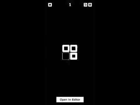
At its core, the puzzle game consists of a grid of squares that can be either black or white. You can toggle a square's color by pressing it, but doing so also toggles the colors of its adjacent squares (top, bottom, left, and right). Your objective is to turn all the squares to black by carefully choosing which squares to press.
The challenge here lies in the interaction of squares. Each move not only affects the square you press but also impacts its neighbors, creating a domino effect that must be carefully managed. Therefore, your strategy should account for multiple steps ahead, as the outcome of one press can alter the state of the entire grid.
The puzzle we're tackling isn't just a fun game; it's built on a fascinating mathematical structure, and its solution hinges on a few key properties of the system. Let’s explore the mathematical concepts behind the puzzle, focusing on the following:
- Inversion of Actions: Each action is its own inverse.
- Commutativity of Actions: The order of actions doesn’t affect the resulting configuration.
- Optimization of Actions: The minimum number of actions to solve the puzzle, initially found through brute force, can now be efficiently solved by reinforcement learning.
- Solvability: While not every state is solvable, all solvable states can be transformed into one another.
One of the most important properties of this puzzle is that pressing a square (an action) is self-inverse. This means that if you press the same square twice, the grid will revert to its original configuration.
Let’s break this down:
- Each action affects the color of the square you press and its neighboring squares (top, bottom, left, and right).
- If a square starts white, pressing it turns it black, and pressing it again turns it back to white.
- Similarly, the neighboring squares also toggle between black and white with each press.
Mathematically, this can be represented as a binary operation. If we treat the color of each square as a binary value (0 for white, 1 for black), then each press can be seen as flipping the binary value of the selected square and its neighbors.
Another important feature of the puzzle is that the order of actions doesn’t matter. In mathematical terms, this is known as commutativity.
In a typical puzzle game, the sequence in which you perform actions can lead to different outcomes. However, in this case, no matter the order of pressing squares, the final configuration of the grid will be the same.
- For example, pressing square A, then square B, yields the same result as pressing square B, then square A.
- This is because each action only affects the color of the square you press and its immediate neighbors. The interdependencies of the colors are such that you can perform the same set of actions in any order and still reach the same solution.
This commutative property significantly reduces the complexity of the problem, as it removes the need to account for the exact sequence of moves. The puzzle's state is only determined by which squares have been pressed, not in which order.
Originally, the minimum number of moves required to solve any given state in the puzzle was determined using brute-force breadth-first search (BFS). BFS explores all possible states and systematically finds the shortest path to the solution. While this approach guarantees the optimal solution, it’s computationally expensive and impractical for larger grids or more complex configurations.
With reinforcement learning (RL), we’ve taken a different approach that still guarantees an efficient solution but with less computational overhead. In this case, the RL agent is trained on a single state of the puzzle for 2x2 and 3x3 graph space and learns a policy that allows it to solve any other state in the same graph space.
- Single State Training: The agent is initially trained on a single state, which means it only needs to learn the optimal moves for this particular configuration.
- Generalization to All States: Once the agent has learned the optimal policy for this single state, it can then apply the same learned strategy to any solvable configuration within the same graph space (i.e., a graph with the same nodes and edges, but with different initial color configurations).
This generalization is possible because all solvable states can be transformed into one another. The RL agent doesn’t need to memorize solutions for every possible state. Instead, it learns to navigate the space of solvable states by understanding the relationships between them and applying the same strategy, no matter the initial configuration.
Not every configuration of the grid is solvable. For example, there may be certain initial conditions where it’s impossible to turn all squares black, no matter how many moves you make. However, all solvable states are interconnected—meaning that every solvable configuration can be reached from any other solvable configuration.
This property is crucial because it means that once the RL agent learns how to solve one state, it can transform any other solvable state into the solution through a series of actions. This connectivity of solvable states allows the agent to generalize its learned policy to all configurations within the same space.
Mathematically, we can think of the graph of all possible states as a graph of interconnected nodes, where each node represents a specific configuration of the puzzle, and edges represent valid moves. Solvable states form a connected component within this graph, and the agent can navigate through this space by applying actions based on its learned policy.
By combining the self-inverse property of actions, the commutative nature of the puzzle, and the connectedness of solvable states, the RL agent can efficiently solve any solvable puzzle configuration. The agent’s training process allows it to learn the optimal strategy from a single state, and it can then generalize this knowledge to navigate the graph of all solvable states.
This marks a significant leap from brute-force methods like BFS, offering a more scalable and efficient approach to solving the puzzle. The RL agent does not need to search through every possible state; instead, it relies on the generalizations it has learned through its training. As a result, it can solve puzzles faster and with fewer computational resources.
Reinforcement learning is a branch of machine learning where an agent learns how to achieve a goal by interacting with an environment. The agent receives feedback in the form of rewards based on its actions, which helps it learn the most effective strategies over time.
In our case, the environment consists of the grid of squares, and the goal is to toggle them all to black. The agent learns through trial and error, selecting actions (pressing squares) and receiving rewards or penalties based on the state of the grid after each action.
Here’s a breakdown of how reinforcement learning, specifically Q-learning, is used to solve this puzzle game.
The first step is to model the puzzle game as an environment. Each square is represented as a node in a graph, and the edges between them represent their adjacency. The environment tracks the state of each square (whether it is black or white) and updates the state whenever a square is pressed.
import networkx as nx
import matplotlib.pyplot as plt
import numpy as np
import random
from datetime import datetime

class GraphEnvironment:
    def __init__(self, graph, goal_product=1):
        self.graph = graph
        self.goal_product = goal_product
        self.state = self.get_state()
        self.initial_state = self.get_state()

    def initial_state(self):
        """ Initialize the state: a dictionary of node weights. """
        return {str(node):  self.graph.nodes[node]['color'] for node in self.graph.nodes}

    def set_state(self, target_state):
        self.state = target_state
        for node in self.graph.nodes:
            self.graph.nodes[node]['color'] = target_state[str(node)]

    def change_color(self, node):
        self.graph.nodes[node]['color'] = 1 - self.graph.nodes[node]['color']

    def apply_action(self, action):
        """ Apply an action (modify node weights) and return the new state. """
        self.change_color(action)
        for node in self.graph.neighbors(action):
            self.change_color(node)
        self.state = self.get_state()
        return self.state

    def get_state(self):
        return {str(node):  self.graph.nodes[node]['color'] for node in self.graph.nodes}

    def get_reward(self, state):
        """ Reward is based on how close the product of node weights is to the goal. """
        product = 1
        for color in state.values():
            product *= color
        if product == self.goal_product:
            return 100
        elif product == 0:
            return -100
        else:
            return -10

    def is_done(self, state):
        """ Check if the goal is reached (product == 1) or the game should end. """
        product = 1
        for color in state.values():
            product *= color
        return product == self.goal_product

    def get_possible_actions(self):
        """ Return a list of all possible actions. """
        return [node for node in self.graph.nodes]
The environment tracks the color of each node and updates the state after every action. The get_reward() function provides feedback to the agent based on how close it is to the goal, rewarding it when all squares turn black.
Q-learning is an off-policy RL algorithm that helps an agent learn the best actions by estimating the long-term value (reward) of each action in each state. In our game, the agent learns which square to press to get closer to the goal.
The Q-learning algorithm maintains a Q-table that stores the expected future rewards for each state-action pair. During training, the agent explores different actions and updates the Q-table based on the rewards it receives.
import random

class QLearningAgent:
    def __init__(self, graph_environment, alpha=0.1, gamma=0.9, epsilon=0.1):
        self.env = graph_environment
        self.alpha = alpha  # Learning rate
        self.gamma = gamma  # Discount factor
        self.epsilon = epsilon  # Exploration factor
        self.q_table = {}  # Q-table, key = state, value = action-value dictionary

    def choose_action(self):
        """ Choose an action using epsilon-greedy approach. """
        state = self.env.get_state()
        state_tuple = tuple(sorted(state.items()))
        if random.random() < self.epsilon:
            return random.choice(self.env.get_possible_actions())
        else:
            if state_tuple not in self.q_table:
                self.q_table[state_tuple] = {action: 0 for action in self.env.get_possible_actions()}
            return max(self.q_table[state_tuple], key=self.q_table[state_tuple].get)

    def learn(self, action, reward, next_state):
        """ Update the Q-table based on the action taken and the received reward. """
        state = self.env.get_state()
        state_tuple = tuple(sorted(state.items()))
        next_state_tuple = tuple(sorted(next_state.items()))
        if state_tuple not in self.q_table:
            self.q_table[state_tuple] = {action: 0 for action in self.env.get_possible_actions()}
        if next_state_tuple not in self.q_table:
            self.q_table[next_state_tuple] = {action: 0 for action in self.env.get_possible_actions()}

        max_next_q_value = max(self.q_table[next_state_tuple].values())  # Maximum Q-value for next state

        # Update Q-value using the Q-learning formula
        self.q_table[state_tuple][action] = self.q_table[state_tuple][action] + self.alpha * (
            reward + self.gamma * max_next_q_value - self.q_table[state_tuple][action])

    def train(self, episodes=1000):
        """ Train the agent over multiple episodes. """
        for episode in range(episodes):
            self.env.set_state(self.env.initial_state)
            done = False
            while not done:
                action = self.choose_action()
                next_state = self.env.apply_action(action)
                reward = self.env.get_reward(next_state)
                done = self.env.is_done(next_state)
                self.learn(action, reward, next_state)
                state = next_state
            if episode % 500 == 0:
                print(f"Episode {episode}: Training...")
The agent explores the environment by choosing actions with an epsilon-greedy strategy, meaning it either explores randomly or exploits the best-known action. Over time, it updates the Q-table to favor actions that lead to higher rewards (more squares turned black).
# Parameters 2x2 graph
rows = 2
cols = 2

G = nx.Graph()

for row in range(rows):
    for col in range(cols):
        node = (row, col)
        G.add_node(node)
        if (row + col) % 2 == 0:
            G.nodes[node]['color'] = 1
        else:
            G.nodes[node]['color'] = 0

for row in range(rows):
    for col in range(cols):
        node = (row, col)
        if col + 1 < cols:
            G.add_edge(node, (row, col + 1))
        if row + 1 < rows:
            G.add_edge(node, (row + 1, col))


env = GraphEnvironment(G)
agent = QLearningAgent(env)
start_time = datetime.now()
agent.train(episodes=3200)
print(f"Training done. Total time spent: {datetime.now() - start_time}")def draw_graph(G, pos):
node_colors = ['black' if G.nodes[node]['color'] == 1 else 'white' for node in G.nodes()]
fig = plt.figure(figsize=(1.6 * rows, 1.6*cols))
nx.draw(G, pos, with_labels=True, node_size=20000, node_shape='s', node_color=node_colors, font_size=10, font_weight='bold', edge_color='gray')
fig.set_facecolor('skyblue')
plt.title("2x2 Puzzle")
plt.show()
def test_agent(agent, starting_state =None, max_steps=10):
"""
Function to test the agent's performance after training.
:param agent: The trained Q-learning agent
:param max_steps: Maximum number of steps (actions) to test before stopping
:return: Success (True/False), number of steps taken, and the final state
"""
if starting_state is None:
agent.env.state = env.set_state(env.initial_state)
else:
agent.env.state = env.set_state(starting_state)
done = False
steps_taken = 0
pos = {(row, col): (col, -row) for row in range(rows) for col in range(cols)}
draw_graph(G, pos)
while not done and steps_taken < max_steps:
action = agent.choose_action()
next_state = agent.env.apply_action(action)
reward = agent.env.get_reward(next_state)
done = agent.env.is_done(next_state)
print( f"Action = {action}")
draw_graph(G, pos)
state = next_state
steps_taken += 1
if done:
print(f"Goal reached in {steps_taken} steps!")
else:
print(f"Goal not reached within {max_steps} steps.")
return done, steps_taken, state
# Parameters
rows = 3
cols = 3

G = nx.Graph()

for row in range(rows):
    for col in range(cols):
        node = (row, col)
        G.add_node(node)
        G.nodes[node]['color'] = 0

for row in range(rows):
    for col in range(cols):
        node = (row, col)
        if col + 1 < cols:
            G.add_edge(node, (row, col + 1))
        if row + 1 < rows:
            G.add_edge(node, (row + 1, col))


env = GraphEnvironment(G)
agent = QLearningAgent(env)
start_time = datetime.now()
agent.train(episodes=32000)
print(f"Training done. Total time spent: {datetime.now() - start_time}")

The results of the experiment show that the agent was able to effectively solve simple tasks requiring 1-2 steps, successfully identifying and applying the optimal actions within the constraints of the environment. However, as the complexity of the tasks increased, particularly in cases requiring more steps, the agent struggled to generate the desired solutions. This limitation was mainly due to the maximum number of actions constraint, which restricted the agent from exploring the full space of possible actions. As a result, the agent was unable to reach optimal solutions in more intricate scenarios, highlighting the need for further adjustments in action exploration or relaxation of the action limit to improve performance on more complex tasks.
Potential Improvements:
- Extended Training: Training the agent for a longer period could help it better explore and adapt to complex tasks.
- Adjusting the Reward Mechanism: Tweaking the reward structure could better guide the agent's decision-making process.
Would you consider increasing the reward for reaching intermediate states or achieving smaller milestones, or would you lean toward increasing the punishment for suboptimal actions? What would be your strategy to improve the agent's performance?
Thanks!
Zeliha Ural Merpez